
| En Français | Home/Contact | Billiards | Hydraulic ram | HNS | Relativity | Botany | Music | Ornitho | Meteo | Help |
Scientific approach aims to produce verifiable knowledge through a logical progression of steps.
Systemic modeling represents an essential step in this process, allowing us to understand a phenomenon as a system.
Written expression modeling extends this logic by ensuring a universal and unambiguous understanding of the ideas expressed.
D1.1. Scientific approach :
The standard scientific approach taught in France (OHERIC model) comprises the following steps :
1. Observation (O) :
Precise measurement of a phenomenon.
2. Hypothesis (H) :
Systemic modeling and formulation of the simplest theory accounting for all observed facts, from which testable hypotheses are derived.
3. Experiment (E) :
Experimentation and testing of the formulated hypotheses.
4. Results (R) :
Collection and organization of the data obtained from the experiment.
5. Interpretation (I) :
Comparison of the results with the hypotheses and also with existing theories.
6. Conclusion (C) :
Synthesis of the results with validation or rejection of the hypotheses.
7. Communication (addition to the OHERIC model) :
Communication of the results for peer review and possible criticism.
Warning : All criticism must be constructive to be admissible, that is, factual, without value judgments, ironic or disrespectful remarks, in short, worthy of the critic.
8. Application (addition to the OHERIC model) :
Use of the theory to predict or reproduce the phenomenon.
D1.2. Systemic modeling :
The systemic modeling is a stage of the scientific approach which consists in describing physical phenomena in the form of systems. The challenge is to find the right level of model : neither too simple to take into account all the physical observations, nor too complex to set the model parameters from these observations.
Systemic modeling also aims to divide systems into subsystems in an optimal way according to four main principles of systemes urban planning :
1. "Divide to conquer" or modularity principle. The goal is to cut the system into subsystems of optimal size and each having its autonomy of exploitation and use.
The temporary unavailability of a subsystem does not prevent the other subsystems from operating.
2. "Group to simplify" or subsidiarity principle. The goal is to pool what can be pooled and to treat each specificity as a differential relative to the general case.
Complexity is isolated in easily manageable special case subsystems and does not put generic subsystems at risk.
3. "Distribute to better communicate" or reducing adhesions principle. The goal is to minimize the adhesions between subsystems and to compensate by a dynamic cooperation between them.
The data exchanged between subsystems are only created and modified in a single subsystem (notion of proprietary subsystem).
The information exchanges between subsystems are done via standardized interfaces.
4. "Start small but think big" or progressiveness principle. The goal is to provide for an evolution of the system in stages and starting from the existing one.
D1.3. Written expression modeling :
The same text can be interpreted in multiple ways by different readers. This variability stems primarily from the ambiguity of words. For example, the word house can refer to a dwelling, a farm, or a business.
To write a text understood identically by everyone, and therefore inherently beyond criticism, one must strive for writing whose comprehension is independent of cultural context. This remarkable result is achieved when each word possesses a unique semantic value and each sentence expresses an explicit logical relationship.
The fundamental principles of unambiguous communication are as follows (listed in descending order of importance) :
1. Context level. The text must be preceded by its publication date, its author and its purpose, the latter often indicated in the preamble.
2. Structure level. The text must be structured into distinct parts. Two methods exist : The three-level logical structure (introduction, development, conclusion) used to explain in depth or tell a story, and the journalistic structure (summary, details) used to capture attention and inform quickly.
3. Lexical level. Each keyword must be explicitly defined with illustrative examples, either inserted directly into the text, referenced in an appendix, or included in a specialized glossary. This principle ensures that words are understood in the author's intended sense and not according to their cultural or subjective meanings. This applies particularly to common nouns and adjectives. Lexical precision can be achieved through two complementary methods :
- Comprehensive definition of the word by context or specific characteristics. The meaning of the word must be anchored in a context or by grammatical or semantic clarification. For example, the sentence "Show hypnosis is safe" contains an ambiguity related to the word "safe" which can be interpreted by the reader either absolutely ("no danger") or relatively ("frequent absence of danger"). To resolve the ambiguity, the sentence can be reformulated as follows : "Show hypnosis is safe in the majority of cases"
- Formal definition through hierarchical decomposition of the word. The word is described in smaller, well-defined constituent units, following a tree-like structure. For example, the sentence "Birdsong is a sound signal resulting from the repetition of the same phrase" is syntactically correct but imprecise. The word "phrase" must be formally defined as follows : a Phrase is a succession of Words, each ending in a Silence ; a Word is an uninterrupted succession of Syllables ; a Syllable is a sound produced in a single vocalization. Thus, the song of the the Turkish turtle dove is characterized by the Phrase "rou.rouhh rou " composed of two Words "rou.rouhh" and "rou", the first Word itself being composed of two Syllables "rou" and "rouhh".
4. Syntactic level. Sentences must be structured according to rigorous syntax and appropriate punctuation. By combining the principles 2 and 3, verbs acquire a more precise meaning. They become logical operators linking clearly defined and identified concepts.
5. Coherence level. The text must not present any internal contradictions, either between sentences or with the associated glossary.
6. Readability level. The text should be organized into clearly identified sections and paragraphs, with evocative titles and subtitles. Sentences should be short and simple, ideally with only one idea per sentence. The progression of ideas should follow a clear logic, moving from the general to the specific.
7. Traceability level. Every idea must be linked to a reliable source, an established rule, or a clear prior reference to prevent the spread of unsourced or erroneous information.
8. Neutrality level. The writing must be devoid of value judgments or appeals to emotion. The sentences should describe, not convince.
9. Conciseness level. Superfluous or non-essential details must be removed to retain only the fundamental concepts, which makes the text impactful.
10. Dual reading level. Highly technical or specialized words should be placed in parentheses immediately after the main word. This principle aims to offer two levels of reading : one for the uninitiated or hurried reader, and the other for the specialist.
11. Analogy level. Abstract ideas benefit from being accompanied by a concrete and familiar image (metaphor). A common example related to teamwork : "Collaborating effectively is like cooking together following a recipe."
|
Conclusion : Word choice, the cornerstone of communication, shapes understanding and conditions all other principles. Yet each word carries within it a unique story, made up of experiences and perceptions specific to each individual. It is therefore essential to choose words with great care when expressing oneself (in writing or orally) and, when receiving them, to suspend any automatic interpretation, in order to guarantee open and constructive communication with others. |
D2.1. Definition :
The Digital Optical Disk (DON) is a removable flat disk used to store digital data in the fields of computers, audio and video.
The best known disks are CD, DVD and BD :
The acronym CD, DVD or BD is followed by the burning mode : ROM (Read-Only Memory) for read-only disk, ±R (Recordable) for disk that can only be written to once, ±RW (Rewritable) or ±RE for rewritable disk.
The acronym ± of burning mode corresponds to two different DVD standards, the old players not being compatible with the + standard which is more recent.
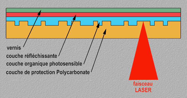
D2.2. Constitution :
A digital optical disk is a stack of several layers (see Figure above) :
Data is written in the base layer for ROM, in the dye layer for ±R and in the reflective layer for ±RW, on a spiral-shaped track that is almost 5 km long for disks CD, from the center outwards.
Optical reading is binary (0 or 1). The information is made up of micro-pits and lands. Any state change (land to micro-pit or vice versa) is translated by a '1', and all the lengths of lands and micro-pits by '0'.
D2.3. Lifetime :
The objective lifetime of a digital optical disk ranges from 2 years to 20 years, and sometimes longer if all precautions are taken. It strongly depends on the choice of media, the use conditions and the storage conditions of the disk.
D2.4. Choice of media :
D2.5. Use :
D2.6. Conservation :
D2.7. Sources relating to Digital optical disk :
Wikipedia - Disque Compact.
Wikipedia - DVD.
Wikipedia - Disque Blu-ray.
Level - Quelles sont les différences entre un CD et un DVD ?.
Infobidouille - La question technique 6 : CD, DVD, BLU-RAY, RW... Comment ça marche les supports optiques ?.
FISTON production - Inquiétudes sur la durée de vie des DVD enregistrables.
Maxicours - Stockage optique.
expert multimedia - Caractéristiques techniques d'un DVD.
Chaumette O., AGIR/PHYSIQUE/CHAP 20 - Le principe de la lecture d'un disque optique (CD, DVD, BluRay...).
Gouvernement du Canada - Durabilité des CD, des DVD et des disques Blu-ray inscriptibles.
Centre de conservation du Québec - Critères de choix d'un disque optique, guide d'entretien et de manipulation.
SOSORDINATEURS - Quelle est la durée de conservation des CD, DVD et Blu-Ray.
VERBATIM - Les différences significatives de performance entre les couches réfléchissantes en argent et en aluminium soulignent l'importance de savoir ce que vous achetez.
Que Choisir - Durée de vie des DVD - Conseils.
Ballajack - Durée de vie d'un CD ou DVD gravé, comment les conserver ?.


Purchasing an electric car, whether 100 % electric, hybrid or hydrogen, requires careful consideration.
These different types of vehicles have the following advantages and disadvantages compared to a conventional car with a thermal engine (petrol or diesel).
D3.1. The 100 % electric car
D3.2. The hybrid car
D3.3. The hydrogen car
D3.4. Synthesis :
|
Statistics : At the end of 2024, the French electric passenger car fleet (excluding light commercial vehicles) represents approximately 8 % of the total fleet, broken down as follows : 2.2 % (100 % electric), 1.5 % (plug-in hybrids) and 4.4 % (non-rechargeable hybrids). Purchasing a 100 % electric or hybrid vehicle : Many buyers focus on the purchase price, short-term fuel savings, and tax or environmental benefits. But you also need to consider : - Costs beyond 8 years, including possible battery replacement. - Underestimated expenses, such as as additional costs (insurance, tire replacement, repairs, software updates) and cost of recharging the battery, particularly at fast charging stations. - The financial risk that a minor accident could damage the battery (for example, a simple collision with a sidewalk) and result in the vehicle being classified as a wreck (damage to the electrical system, impact on sensitive areas of electric vehicles, total or partial immersion in water). - The concerns about the autonomy of the 100 % electric car and the network of charging stations. - The few number of garages qualified to work on the electrical part of electric vehicles. In rural areas in France, the garage offer tends to split between small garages focused on thermal engines, and specialized centres qualified for electric vehicles. The former often adopt an intermediate organization : a single technician, trained to isolate electric vehicles (at an average cost of about 700 euros), secures the intervention, allowing the other mechanics to work only on parts outside the high-voltage zone. For low-income households, two major obstacles remain : the high purchase price and the risk of being classified as a wreck after even a minor collision. Thus, the appeal of a 100 % electric or hybrid car is based more on environmental concerns, particularly the reduction of CO2 emissions, than on strictly short- or long-term economic logic. An informed decision therefore requires a complete analysis of all these aspects in order to allow buyers to make an objective choice adapted to their situation. Note that electric cars with higher ground clearance, such as electric SUVs or crossovers, offer better protection against the two major risks for electric vehicles : underbody impact and accidental immersion. Purchasing a hydrogen vehicle : Purchasing a hydrogen vehicle is now more relevant for professional fleets than for individuals due to a market that is still developing. The main obstacles include : - a high purchase price, - an insufficient network of hydrogen refueling stations, - as for electric or hybrid cars, the financial risk that a accident could damage the battery, or even the hydrogen tank or fuel cell, and result in the vehicle being classified as a wreck. European regulation : Two regulations are important : 1. From 2035, by European regulation published in the EU Official Journal on 25 April 2023 and entered into force on 15 May 2023 [EUR] : - The sale of new cars with combustion engines (petrol, diesel and current hybrids), such as passenger cars or light commercial vehicles, will be banned in the European Union. Only "zero-emission" vehicles, such as 100 % electric cars or those using synthetic fuels (e-fuels) or hydrogen (FCEV), will be allowed to be sold. - The ban does not apply to the second-hand market. - Combustion-engine cars already in circulation are not affected and may continue to be used and resold. The hybrid car market, despite its current success, is therefore set to gradually disappear by 2035, unless they achieve exceptional performance in electric mode. The hybrid car thus appears to be a simple transitional stage towards all-electric. 2. The Regulation resulting from the early review clause (Council Decision EU 2026/514), published in the EU Official Journal on 3 April 2026, and entering into force on 6 April 2026, lowers the emission reduction target to 90 % for 2035 (instead of 100 %), thereby allowing internal combustion and hybrid engines to remain on the market, provided that the remaining 10 % is offset by biofuels, synthetic fuels (e-fuels), or low-carbon steel. First aid : For a witness to an accident, the additional actions to take on an accident-damaged electric, hybrid or hydrogen vehicle are as follows : - Identify and report the type of vehicle to the emergency services (vehicle make, and specific engine/motorization logos if visible at the rear) because these vehicles present specific risks, particularly concerning the high-voltage battery, the high-pressure hydrogen tank and fire management. - Maintain a safety distance of at least 30 metres around the accident-damaged vehicle to avoid any danger of electric shock, explosion or fire. - Do not use water to extinguish a battery fire without the advice of the fire department. In the rare event of a lithium-metal battery fire, the use of water may make the fire worse. |
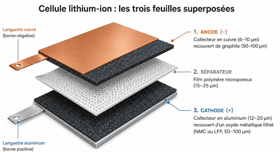
D3.5. Composition of a lithium-ion battery
A lithium-ion battery used in an electric vehicle is an assembly of several hundred or thousands of individual cells.
Each cell consists of an assembly of three stacked layers with a total thickness of approximately 0.2 to 0.4 mm (see Figure 3 above, cf. [CHA]) :
1. The anode (negative electrode) is a copper metal current collector (6 to 10 µm) coated on both sides with graphite (50 to 100 µm).
2. The separator is a microporous polymer film made of polyethylene or polypropylene (15 to 25 µm) that electrically insulates the electrodes while allowing lithium ions (Li+) to pass through.
3. The cathode (positive electrode) is an aluminum metal current collector (12 to 20 µm) coated on both sides with a lithiated metal oxide (NMC or LFP, 50 to 100 µm).
The electrolyte is an organic liquid containing a lithium salt, which permeates the pores of the separator and both electrodes. It enables the transport of Li+ ions between the anode and cathode, while electrons circulate through the external electrical circuit.
Each current collector has a conductive tab protruding from the cell to ensure external electrical connection : copper for the negative terminal, aluminum for the positive terminal.
This "sandwich" of layers exists in three distinct geometric configurations :
- Cylindrical : The three layers are wound into a spiral (jelly roll) after stacking. The electrodes can reach several meters in length for only a few centimeters in width.
- Pouch : The electrodes are stacked in rectangular sheets and encapsulated in a flexible laminated aluminum pouch.
- Prismatic : The electrodes are stacked and inserted into a rigid metal casing, forming a compact block a few centimeters thick.
D3.6. Sources relative to electric cars :
[ADE] ADEME, Mondial de l'automobile : l'ADEME publie son avis sur le véhicule électrique : une batterie de taille raisonnable assure une pertinence climatique et économique.
[AUJ1] L'auto-journal, Voitures électriques : quel est le coût des réparations ?.
[AUJ2] L'auto-journal, Véhicules électriques et entretiens : un vrai cauchemar ?.
[AUM] L'Automobile Magazine, Les voitures électriques sont-elles 3 fois plus dangereuses pour les piétons ?.
[AUT] Auto, Attention, les voleurs s'attaquent aux batteries des véhicules hybrides.
[CAP1] Capital, Accidents de la route : dans quels cas votre voiture est-elle jugée irréparable ?.
[CAP2] Capital, Automobile : découvrez pourquoi réparer un véhicule électrique coûte plus cher !.
[CEN] La Centrale, Quand la batterie flanche : dites adieu à votre voiture électrique et direction la casse !.
[CHA] ChatGPT, le moteur d'Intelligence Artificielle développé par OpenAI.
[CNR] CNRS Le journal, Les défis de la voiture à hydrogène.
[ECO] Ecoconso, Voiture électrique : ses avantages et inconvénients.
[EDM] Les éditions du moteur, Voiture électrique : Le désamour inattendu qui touche 30 % des propriétaires.
[EUR] EUR-Lex, Règlement (UE) 2023/851 du Parlement européen et du Conseil du 19 avril 2023 modifiant le règlement (UE) 2019/631 en ce qui concerne le renforcement des normes de performance en matière d'émissions de CO2 pour les voitures particulières neuves et les véhicules utilitaires légers neufs conformément à l'ambition accrue de l'Union en matière de climat.
[MAC] Machines Production, Voitures électriques : l'épineux problème des batteries après un accident.
[NUM] Numerama, Au moindre accident votre voiture électrique peut finir au rebut à cause de sa batterie.
[PER] Perplexity, le moteur d'Intelligence Artificielle développé par Perplexity AI.
[PRE] Pressecitron, Une voiture électrique coûte-t-elle vraiment moins cher à l'usage qu'une thermique ?.
[QUE] Que choisir, Comment choisir une voiture hybride.

D7.1. Introduction :
Quantum physics is a fundamental branch of physics that describes the universe at the microscopic level of atoms, molecules, and elementary particles, taking into account their dual nature of wave and particle.
It differs from classical physics in its counterintuitive concepts such as energy quantization, wave-particle duality, superposition of states, quantum indeterminism, and quantum nonlocality.
These concepts have given rise to many modern technologies such as electronics, quantum computers, medical imaging, and nanotechnology.
Albert Einstein played a major role in the development of quantum physics, notably through his explanation of the photoelectric effect (1905), the quantization of atomic oscillators (1907), wave-particle duality for light (1909), stimulated emission (1917) and the EPR paradox (1935).
Although he always recognized the validity and effectiveness of quantum formalism, he opposed the probabilistic interpretation of Niels Bohr and the Copenhagen School. Einstein defended a simultaneously deterministic and local view of the quantum world, believing in the existence of "hidden variables" that could explain quantum phenomena more completely.
However, subsequent experiments, notably those of Alain Aspect in 1982 [ASP], contradicted this view by demonstrating that quantum mechanics violates quantum locality regardless of whether it is deterministic or not.
Quantum mechanics constitutes the theoretical and mathematical foundation which formalizes the fundamental principles governing quantum physics.
D7.2. Standard model of particles physics (reminder) :
See Relativity - Lexicon : Standard model of particles physics.
D7.3. Fundamental principles :
The fundamental principles governing quantum physics are as follows [CHA][PER], listed in chronological order of discovery.
1. Quantization of Energy (Max Planck, 1900, Albert Einstein, 1905-1917)
Energy can only take discrete values, called quanta, and not continuous values.
This principle was gradually established and extended as follows :
- Blackbody radiation (Max Planck, 1900, and Nobel Prize in Physics in 1918) : For an atom, the energy difference E between two energy levels is given by : ΔE = h ν, where h is Planck's constant and ν is the frequency associated with the transition.
- Photoelectric effect (Albert Einstein, 1905, and Nobel Prize in Physics in 1921) : Einstein extends Planck's quantization to light itself.
- Quantization of atomic oscillators (Albert Einstein, 1907) : Einstein applies quantization to the vibrations of atoms in a solid.
- Stimulated emission (Albert Einstein, 1917) : Einstein completes the description of the interaction between light and matter in which an incident photon causes an atom to de-excite, emitting a second photon of the same direction, frequency, and polarization.
Confirmation of the quantization introduced by Planck (1900) : Franck and Hertz's experiment (1914) showed that accelerated electrons lost energy in discrete amounts during collisions with mercury atoms.
2. Wave-Particle Duality (Albert Einstein, 1909, Louis de Broglie, 1924)
Quantum objects, such as electrons and photons, exhibit both particle and wave properties depending on the experimental conditions.
The wavelength λ associated with a particle with momentum p is given by : λ = h/p
For a non-relativistic particle with mass m and velocity v, we have: p = m v.
For a photon with energy E, we have : p = E/c
This principle was established in two steps as follows :
- Einstein lays the foundations of wave-particle duality for light (1909).
- De Broglie generalizes this concept to all matter (1924, and Nobel Prize in Physics in 1929).
Confirmation : Davisson-Germer's experiment (1927) demonstrated the diffraction of electrons by a nickel crystal, thus confirming their wave nature.
3. Statistics of Bosons and Fermions (Satyendra Nath Bose and Albert Einstein, 1924, Enrico Fermi and Paul Dirac, 1926)
Bosons (with integer spin, like the photon) follow Bose-Einstein statistics for their collective behavior.
Fermions (with half-integer spin, like the electron) follow Fermi-Dirac statistics for their collective behavior.
Confirmations :
- Bose-Einstein condensate (Eric Cornell and Carl Wieman, 1995, and Nobel Prize in Physics in 2001) by cooling rubidium atoms (bosons).
- Pauli blockade (MIT, 2021) by cooling a lithium-6 gas cloud (fermions).
4. Pauli Exclusion (Wolfgang Pauli, 1925, and Nobel Prize in Physics in 1945)
Two identical fermions, like electrons, protons, or neutrons, cannot simultaneously occupy the same quantum state in the same system.
This principle is fundamental to explaining the electronic structure of atoms, particularly the distribution of electrons in atomic shells and subshells, which leads to the structure of the periodic table of elements.
Confirmations :
- Analysis of the Zeeman effect (1927-1930).
- Study of electronic band structure and nuclear physics (1930-1940).
5. Quantum Superposition (collective, 1926)
A quantum system exists in an indeterminate global state as a superposition of several states simultaneously until a measurement is made. After the measurement, the system collapses into a single state corresponding to the observed result.
Confirmation : Clinton Davisson and Lester Germer's experiment (1927) on the diffraction of electrons by a crystal.
|
Formalization [PER][CHA] :
It applies to any quantum phenomenon, such as the Stern-Gerlach experiment (see below) for the discrete case and the calculation using the continuous Schrödinger method in the continuous case. The wave function Ψ(x, t)is an abstract representation containing all possible information about the state of a particle or quantum system at a given instant. It allows us to calculate the probabilities of different measurement outcomes but does not determine with certainty the outcome of a single measurement. It is expressed mathematically in a standard way as the superposition of eigenstates Ψj in the form : - Discrete case : Ψ(x, t) = ∑j [cj Ψj(x, t)] where j is the index that numbers the different eigenstates Ψj - Continuous case : Ψ(x, t) = ∫R [c(k) Ψk(x, t) dk] where k is a continuous variable. where the variable x can be a position, a volume, a momentum, an energy, etc. Given the normalization condition (see below), the unit of Ψ(x, t) is dimensionless in the discrete case and the square root of the inverse of the unit of x in the continuous case (for example, Ψ(x,t) has the unit of m-1/2 for x expressed in meters). The eigenstates Ψj are characteristic modes of the system for which the measurement of an observable always gives the same result with a probability of 100 %. These modes are analogous to : - Discrete case : the specific tuning frequencies of a radio, where the observable is the radio frequency, - Continuous case : the specific vibration modes of a taut string, where the observable is the vibration frequency. Each eigenstate Ψj(x, t) is expressed in the complex form : Ψj(x) e-i Ej t/h' with a non-temporal part Ψj(x) that is a solution to the stationary Schrödinger equation and a phase part that depends on time t. Ej is the energy associated with the eigenstate Ψj and h' is the reduced Planck constant. The coefficients cj are the probability amplitudes associated with each eigenstate. They are expressed in the complex form : |cj| ei θj where |cj| is the module of coefficient and θj is the initial phase angle in the complex plane. The determination of the cj coefficients is essentially experimental. The |cj| moduli are obtained by statistical measurements on many copies of the system. Relative phases require more advanced techniques such as quantum tomography. More generally, regardless of the type of quantum state (eigenstate or superimposed), the probability amplitude is a complex coefficient associated with each eigenstate of the wave function, allowing the calculation of the probability of observing a specific outcome during a measurement. This concept was introduced in 1926 by Max Born [BOU], who showed that the wave function Ψ could not be interpreted directly as a probability because this would violate the rules for calculating probability for compound events. He proposed that the probability of observing a given state be given by the square of the modulus of the probability amplitude, i.e. |Ψ|2 Hence the following four cases : 1. Discrete case of an eigenstate Ψj : The state of the system is Ψj, with a probability amplitude of 1 for Ψj and a probability of 1 of observing state Ψj 2. Continuous case of an eigenstate Ψj : The state of the system is Ψj(x, t), with a probability amplitude Ψj(x, t) and a probability density ρ(x, t) = |Ψj(x, t)|2 giving the probability of finding at time t the value x of the measured variable. 3. Discrete case of a superposition of eigenstates : The state of the system is a superposition Ψ(x, t) = ∑j cj Ψj(x, t), with a probability amplitude cj for each eigenstate Ψj and a probability Pj = |cj|2 of observing state Ψj 4. Continuous case of a superposition of eigenstates : The state of the system is a superposition Ψ(x, t) = ∫R c(k) Ψk(x, t) dk, with a probability amplitude density c(k) for each eigenstate Ψk and a probability density ρ(x, t) = |Ψ(x, t)|2 giving the probability of finding at time t the value x of the measured variable taking into account the effects of quantum interference between the different eigenstates. Note that the probability amplitude is the wave function itself only in the continuous case of an eigenstate (case 2). The normalization condition guaranteeing that the sum of the probabilities is equal to 1 also imposes that : 1. Discrete case of an eigenstate Ψj : ∑i |Ψj(xi)|2 = 1 where xi are the discretization points. 2. Continuous case of an eigenstate Ψj : ∫R |Ψj(x, t)|2 dx = 1 3. Discrete case of a eigenstates superposition : ∑j |cj|2 = 1 4. Continuous case of a eigenstates superposition : ∫R |c(k)|2 dk = 1 or ∫R |Ψ(x, t)|2 dx = 1 Concrete example (Stern-Gerlach experiment, 1922) : The wave function of a silver atom whose spin is in a superposition of states along the z axis can be written : Ψ = c1 |+z> + c2 |-z> where the eigenstates |+z> and |-z> represent the "up" and "down" orientations of the spin along the z axis, respectively. These eigenstates are also the eigenvectors of the spin operator Sz which allows us to measure the projection of the angular momentum on the z axis. This operator is defined by the following matrix : Sz = h'/2 (1 0) (0 -1) where h' is the reduced Planck constant. The eigenvectors associated with this matrix are |+z> = (1, 0)T for the eigenvalue +h'/2 (spin "up"), and |-z> = (0, 1)T for the eigenvalue -h'/2 (spin "down"). These eigenvalues represent the quantization of the angular momentum projections on the z axis, expressed in units of h' The complex coefficients c1 = 1/(21/2) and c2 = i/(21/2) are the probability amplitudes, taking into account both the moduli and the relative phase between the two eigenstates. Therefore, if we perform a spin measurement on the z axis, there is a 50 % chance (= |c1|2) of obtaining the value + h'/2 ("up" state) and a 50 % chance (= |c2|2) of obtaining the value -h'/2 ("down" state). |
6. Quantum Indeterminism (Max Born, 1926, and Nobel Prize in Physics in 1954)
Measurement results are not deterministic, but probabilistic, when the system evolves freely between measurements or is reset to its initial state before each new experiment.
On the other hand, repeated measurements under the same experimental conditions, at very short intervals, give the same result because the system remains in the measured state after the first observation.
Confirmation : Repeated experiments on Young's slits.
Interpretations :
- In the Copenhagen interpretation (Bohr, Heisenberg), this principle calls into question the idea that the properties of a quantum system have an objective reality independent of measurement.
- But other interpretations, such as the de Broglie-Bohm (hidden variable theory) or the Everett (many-worlds) interpretation, challenge this idea while remaining compatible with experimental predictions. To this end, the de Broglie-Bohm interpretation preserves determinism while accepting the principle of quantum nonlocality, and the Everett interpretation avoids the nonlocality problem by proposing that all possible outcomes of a measurement occur simultaneously in distinct universe branches.
7. Quantum Uncertainty (Werner Heisenberg, 1927, and Nobel Prize in Physics in 1932)
There is a fundamental limit to the precision with which certain pairs of physical quantities can be measured, including position and momentum, energy and time, spin and orientation.
For example, the relationship between the uncertainties between position (x) and momentum (p) is given by :
Δx Δp ≥ h'/2
where h' is the reduced Planck constant.
Indirect confirmation : Davisson-Germer's (1927) experiment on electron diffraction by a nickel crystal.
8. Tunneling Effect (George Gamow, 1928)
A particle can penetrate an energy barrier even without the classically required energy. The particle's wave function does not vanish at the barrier but attenuates within it, allowing a non-zero probability of crossing it.
Confirmation : George Gamow's experiment (1928) on the alpha decay of radioactive nuclei.
9. Quantum Entanglement (EPR paradox, by Albert Einstein, Boris Podolsky, Nathan Rosen, 1935)
Two particles are said to be entangled when they form a global quantum system such that measuring the state of one instantly determines the state of the other, regardless of the distance between them.
These instantaneous quantum correlations do not constitute signal transmission, thus escaping the framework of relativistic causality without contradicting it.
Confirmation : Experiments by Alain Aspect (1982, and 2022 Nobel Prize in Physics) that confirmed the predictions of quantum mechanics in violation of Bell's inequalities, thus confirming quantum entanglement [ASP].
10. Path Integral (Richard Feynman, 1948)
A particle traveling from one point to another simultaneously follows all possible paths to reach its destination. Each path is associated with a complex amplitude (modulus and phase), and the probability of finding the particle at a given location is determined by the sum of the amplitudes (with their phases) of all possible trajectories.
This approach is an elegant and powerful reformulation of the Schrödinger equation.
Confirmation : Hitachi's (1989) experiment on single electron interference.
11. Quantum Decoherence (David Bohm, 1951)
A quantum system can lose its coherence (superposition of states) by interacting with its environment, leading to seemingly classical behavior.
Confirmation : Experiments demonstrating the quantum-classical transition (Serge Haroche, 1996, Anton Zeilinger, 2003).
12. Quantum nonlocality (Bell's theorem, by John Bell, 1964)
Quantum objects can exhibit instantaneous correlations over distance. Nonlocality encompasses quantum entanglement by including correlations over time, complex multi-particle systems, interactions between particles and macroscopic objects, and delocalized phenomena without requiring direct interaction.
Confirmation : Experiments by Alain Aspect (1982) confirmed the predictions of quantum mechanics in violation of Bell's inequalities, thus confirming nonlocality [ASP].
13. Quantum Field Theory (collective)
Quantum field theory (QFT) is a theoretical framework unifying quantum mechanics and restricted relativity. It models particles as localized excitations of quantum fields that fill all of space-time, making it possible to explain the creation and annihilation of particles.
Only quantum entanglement escapes the interpretation of causality by its non-local character and the absence of signal transmission, while remaining compatible with the formalism of restricted relativity.
The following contributions are worth mentioning :
- Quantum theory of the electromagnetic field (Paul Dirac, 1927), confirmed in 1930 by the analysis of atomic spectra (notably Alfred Lande and Otto Stern).
- Quantum electrodynamics (QED), describing the interaction between light and matter (Richard Feynman, Julian Schwinger, Sin-Itiro Tomonaga, Freeman Dyson, 1940, and Nobel Prize in Physics in 1965), confirmed in 1947 by Polykarp Kusch and Henry Foley through experiments on the electron's magnetic moment.
- Non-Abelian gauge theories (Yang Chen-Ning and Robert Mills, 1954), providing a theoretical framework for describing non-Abelian interactions such as the weak and strong forces.
- Unification of electromagnetism and the weak force in a standard model (Steven Weinberg, Abdus Salam, Sheldon Glashow, 1960, and Nobel Prize in Physics in 1979), confirmed in 1983 at CERN by the discovery of the W+, W-, and Z0 bosons.
- Higgs boson (Peter Higgs and Fran ois Englert, 1964, and Nobel Prize in Physics in 2013) confirmed in 2012 at CERN by the ATLAS and CMS experiments at the LHC (Large Hadron Collider).
- Quantum chromodynamics (QCD), describing the strong interaction between quarks and gluons (David Gross, Frank Wilczek, David Politzer, 1973, and Nobel Prize in Physics in 2004, Kenneth G. Wilson, 1974), confirmed in 1979 at the DESY (Deutsches Elektron SYnchrotron) center by observing hadronic jets from high-energy particle collisions.
D7.4. Quantum state :
The quantum state of an elementary particle is a complete mathematical description of its observable and probabilistic aspects, distinct from its intrinsic properties.
It also extends to compound systems where interactions, correlations, and entanglement phenomena between particles play a fundamental role.
It is formalized by a state vector |ψ> in an abstract Hilbert space, associated with a wave function ψ(x,t) in a concrete basis, generally the position or momentum basis.
Intrinsic properties are invariant characteristics that define the fundamental nature of the particle, in particular the mass m and the intrinsic quantum numbers.
Observables are measurable physical quantities (such as position x or momentum p) represented mathematically by Hermitian operators (such as X or P).
- Before measurement, the observable is a statistical prediction obtained by calculating the weighted average of the possible outcomes of the measurement, the weights being determined by the probabilities associated with the initial quantum state of the system.
- After measurement, an observable provides a value that corresponds to one of the eigenvalues of the operator associated with the observable.
Operators act on the quantum state of the system (wave function or state vector in a Hilbert space) to calculate information, such as the possible values of observables (eigenvalues) and the probabilities associated with each measurement result. For example :
- the position operator X is the multiplication by x in the form : X(Ψ(x)) = x Ψ(x), allowing the calculation of the average value of the position for this state.
- the kinetic energy operator T acts on the wave function in the form : T(Ψ(x)) = -h'2/(2 m) (d2Ψ(x, t)/dx2)
- the momentum operator P acts by differentiation in the form : P(Ψ(x)) = -i h' dΨ(x)/dx, allowing the calculation of the average value of the momentum for this state.
Note that P can also be written : P = -i h' d/dx
- the Hamiltonian operator H acts on the wave function in the form : H(Ψ(x, t)) = -h'2/(2 m) (d2Ψ(x, t)/dx2) + V(x) Ψ(x, t), allowing the calculation of the total energy of the system.
Note that H can also be written : H = -h'2/(2 m) (d2/dx2) + V(X) = P2/(2 m) + V(X)
- The angular momentum operator J acts on the wave function in the form of a vector product : J(Ψ(x, t)) = r x P(Ψ(x, t)), where r is the position vector and P is the quantized motion operator, allowing the system's angular momentum to be calculated.
- The parity operator π acts on the wave function in the form : π(Ψ(x)) = Ψ(-x), allowing the symmetry of the wave function to be determined with respect to spatial inversion.
- The scaling operators (a+ creation and a annihilation) act on quantum states by adding or removing an excitation particle or quantum.
- The spin operator S acts on spin wave functions in the form of 2x2 Pauli matrices, allowing the intrinsic angular momentum of particles to be described. These matrices are as follows :
σ1 = σx =
(0 1)
(1 0)
σ2 = σy =
(0 -i)
(i 0)
σ3 = σz =
(1 0)
(0 -1)
These matrices verify the property : σ1 σ2 σ3 = i I where I is the Identity matrix.
The eigenvalue is a possible and specific outcome obtained when measuring an observable on a quantum system. It is obtained with certainty if the system is in a corresponding eigenstate, and with a given probability if the system is in a superposition of eigenstates. See Stern-Gerlach experiment.
The eigenvector represents the state of the system when the measurement of an observable yields an eigenvalue. See Stern-Gerlach experiment.
Eigenvectors form a basis for the space of quantum states, allowing all possible configurations of the system to be described.
Measurement probabilities describe how these observables are distributed across their possible value domains in terms of probability density.
They follow Born's rule according to which the probability density ρ is |<Ψj|Ψ>|2, where Ψj is the eigenstate associated with an eigenvalue of the measured observable, that is, the state the system is in immediately after the measurement.
The bra-ket notation <.|.> denotes the Hermitian scalar product which generalizes the classical scalar product to complex vector spaces in the form :
< u|v > = v+.u
where :
u and v = any two column vectors
v+ = adjoint of v = transposed complex conjugate such that v+ = (v*)T
* = complex conjugate operator without transposition
Example : if u = (1 + 2 i, 3)T and v = (4 + 5 i, 6 i)T, then v* = (4 - 5 i, -6 i)T, v+ = (v*)T = (4 - 5 i, -6 i) and < u|v > = v+.u = (4 - 5 i)(1 + 2 i) + (-6 i)(3) = 14 - 15 i
Examples of elementary particles with intrinsic/observable distinction :
Characteristics of the Electron e- :
| Classification : Lepton
| Composition : N/A (Elementary particle)
| Mass (m) = 0.511 MeV/c2
| Intrinsic magnetic moment (μ) = -9.284 10-24 J/T
| Chirality = Right and Left (mixing possible)
| CPT (Charge, Parity, Time) Symmetry : Yes
| Fundamental interactions : electromagnetic, weak and gravitational forces
| Lifetime (τ) = perfectly stable (6.6 1028 years)
| Anti-particle : positron
| Intrinsic quantum numbers :
| | Spin (S) = 1/2
| | Isospin (T3) = -1/2
(for weak isospin)
| | Electric charge (Q) = -1e
| | Color Charge : N/A (particle other than Quark and Gluon)
| | Flavor (Le) : electronic
| | Leptonic number (L) = +1
| | Baryonic number (B) = 0
| Observable quantum numbers :
| | Principal quantum number (n) = strictly positive integer
| | Secondary or azimuthal quantum number (l) = integer from 0 to n
- 1
| | Magnetic quantum number (ml) = integer from -l to +l
| | Magnetic spin quantum number or spin projection (ms) = +1/2 ("up") or -1/2 ("down")
| | Total angular momentum quantum number (j) = |l s|
| | Quantum number or projection of the total angular momentum (mj) = from -j to +j by integer steps
| | Projection of the magnetic moment (μz) = ±9,284 10-24 J/T
| | Parity (P) = accordind to contexte
| | Position, momentum and total energy
Characteristics of the Positron e+ = Anti-electron :
| Classification : Anti-Lepton
| Composition : N/A (Elementary particle)
| Mass (m) = 0.511 MeV/c2
| Intrinsic magnetic moment (μ) = +9.284 10-24 J/T
| Chirality = Right and Left (mixing possible)
| CPT (Charge, Parity, Time) Symmetry : Yes
| Fundamental interactions : electromagnetic, weak and gravitational forces
| Lifetime (τ) = perfectly stable in isolation and short in the presence of matter
| Anti-particle : electron
| Intrinsic quantum numbers :
| | Spin (S) = 1/2
| | Isospin (T3) = +1/2
(for weak isospin)
| | Electric charge (Q) = +1e
| | Color Charge : N/A (particle other than Quark and Gluon)
| | Flavor (Le) : electronic
| | Leptonic number (L) = -1
| | Baryonic number (B) = 0
| Observable quantum numbers :
| | Principal quantum number (n) = strictly positive integer
| | Secondary or azimuthal quantum number (l) = integer from 0 to n - 1
| | Magnetic quantum number (ml) = integer from -l to +l
| | Magnetic spin quantum number or spin projection (ms) = +1/2 ("up") or -1/2 ("down")
| | Total angular momentum quantum number (j) = |l s|
| | Quantum number or projection of the total angular momentum (mj) = from -j to +j by integer steps
| | Projection of the magnetic moment (μz) = ±9,284 10-24 J/T
| | Parity (P) = accordind to context
| | Position, momentum and total energy
D7.5. Quantum calculation methods :
All quantum calculation methods aim to calculate the possible values of observables and their measurement probabilities, but they do so in different ways depending on the application domains. These include :
Warning : It is common to omit certain universal constants from equations, including Planck's constant (h), reduced Planck constant (h'), light speed (c), Identity matrix (I) and gravitational constant (G).
Calculation methods include :
D7.5.1. Non-relativistic Schrödinger-type methods :
These approaches study the time evolution of the quantum state |Ψ> (i.e. wave function Ψ(x, t)), while the observables remain fixed unless the potential V(x, t) is explicitly time-dependent.
They are used particularly in quantum chemistry and follow the Schrödinger equation (1926, Nobel Prize in Physics 1933).
In particular, for a spinless particle of mass m, moving in one-dimensional space and subject to a potential V(x), this equation is written as :
(L1) i h' dΨ(x, t)/dt = -(1/2)(h'2/m)(d2Ψ(x, t)/dx2) + V(x) Ψ(x, t)
where h' is the reduced Planck constant (or Dirac constant = h' = h/(2 π))
and h is Planck's constant (h = 6.626 10-34 J.s).
See example of calculation using the continuous Schrödinger method and example of calculation using the discretized Schrödinger method.
D7.5.2. Relativistic Schrödinger-type methods :
The time evolution of the quantum state is described by wave equations generalizing the Schrödinger equation for particles moving at speeds close to that of light. We can cite :
1. Dirac equation for relativistic particles with spin 1/2 (examples : electron, neutrino).
In particular, for a free particle, this equation is written :
(D1) (i h' γμ dμ - m c I) Ψ = 0
where :
Ψ is the four-component Dirac wavefunction, called spinor, which simultaneously encodes the two spin eigenstates ("up"/"down"), the positive/negative energy solutions (particle/antiparticle), and their relativistic coupling, as follows :
- When momentum p is zero, the four components decompose into two distinct pairs. The first (Φ) encodes the probability amplitudes associated with the spin eigenstates of the particle (e.g., electron). The second (Χ) encodes those of the corresponding antiparticle (e.g., positron).
- As soon as p ≠ 0, the four components describe either a particle (positive energy) or an antiparticle (negative energy). Each individual solution remains a four-component state where spin (described by the Pauli matrices σ) and momentum (vector p) are coupled. One of the pairs encodes the spin eigenstates inherited from the rest frame, modulated by the motion. The other pair encodes their relativistic modification by connecting the two pairs via the total energy E.
m is the mass of the particle at rest.
I is the 4x4 Identity matrix
γμ are specific 4x4 matrices introduced by Dirac, with the index μ ranging from 0 to 3 (0 corresponding to time).These matrices are as follows in standard Pauli-Dirac representation :
γ0 =
(I 0)
(0 -I)
γi =
(0 σi)
(-σi 0)
γ5 = i γ0 γ1 γ2 γ3
(0 I)
(I 0)
in which σi are the 2x2 Pauli matrices and I is the 2x2 identity matrix.
The γμ matrices satisfy the Lorentz group anticommutation relation : {γμ, γν} = γμ γν + γν γμ = 2 gμν I avec gμν = Minkowski metric and I = 4x4 Identity matrix.
dμ are the partial derivatives with respect to the coordinates xμ = (ct, x1, x2, x3) in Minkowski spacetime.
γμ dμ implies a summation over the index μ according to the Einstein summation convention.
The Dirac equation therefore relates the dynamical properties of the particle (energy and momentum via the differential operator i h' γμ dμ) to its proper mass m.
See example of calculation using the Dirac method.
2. Klein-Gordon equation for relativistic particles with spin 0 (example : Higgs boson).
3. Proca equation for relativistic particles with spin 1 (examples : photon, W and Z bosons).
4. Rarita-Schwinger equation for relativistic particles with spin 3/2 (example : gravitino).
5. Generalizations of the Rarita-Schwinger equations for relativistic particles with half-integer spin greater than 3/2.
6. Linearized Einstein equations for the massless spin-2 graviton.
All these equations are invariant under the Lorentz-Poincaré transformation, which makes them compatible with restricted relativity.
However, the interpretation of these equations within the framework of a single-particle theory leads to certain inconsistencies. This is why Quantum Field Theory is essential as a more general and coherent framework.
D7.5.3. Heisenberg-type methods :
These approaches study the temporal evolution of observables, while the quantum state remains fixed.
They are used particularly in quantum operator calculations and quantum field theory. They follow the Heisenberg equation :
(H1) dA/dt = (i/h') [H, A] + DA/Dt
where :
A is the operator A(t) that represents the observable to be studie (e.g., position x(t) or momentum p(t))
H is the Hamiltonian operator of the system
[H, A] is the commutator between H and A, defined by : [H, A] = H A - A H
DA/Dt is the explicit derivative of the operator A in Schrödinger representation, obtained by differentiating only its time part. For example, if A(t) = cos(ω t) X, then DA/Dt = -ω sin(ω t) X
See example of calculation using the Heisenberg method.
D7.5.4. Dirac-type methods :
These approaches combine the time evolution of the quantum state and observables by describing the interactions between relativistic particles within the framework of quantum field theory, particularly in quantum electrodynamics through perturbative calculations and Feynman diagrams.
These approaches use an extended version of the relativistic Dirac equation for a free spin-1/2 particle.
D7.5.5. Advanced Algebraic Methods :
These general methods, based on algebraic tools (matrices, operators, Lie algebras), are used when it is difficult or even impossible to exactly solve the equations of motion, whether differential (Schrödinger-type), matrix (Heisenberg-type) or interactional (Dirac-type).
They allow the solution of simple systems (atoms, small molecules) or more complex systems (large molecules, materials) by providing exact or approximate solutions.
These include :
- Perturbation theory, which is used when the system can be considered a modification of a solvable case.
- Variational method, which provides an estimate of the energies of the bound states by minimizing a trial function.
- Ab initio approaches, which approximately solve the Schrödinger equation from first principles, without resorting to empirical parameters.
D7.5.6. Numerical methods :
These methods are used when it is impossible to obtain analytical solutions to equations.
These include the Monte Carlo method, the finite difference method, and the Lanczos method.
D7.6. Example of calculation using the continuous Schrödinger method :
The following example illustrates quantum computations using the Schrödinger equation.
Assumptions :
We consider a free, non-relativistic, massless, spinless particle located in a one-dimensional infinite potential well.
The time evolution of the wave function Ψ is then given by the Schrödinger equation (relation L1).
(L1) i h' dΨ(x, t)/dt = -(1/2)(h'2/m)(d2Ψ(x, t)/dx2) + V(x) Ψ(x, t)
When we are looking for the eigenstates Ψj of the system (numbered by the index j), the wave function Ψj(x,t) can be decomposed into a stationary spatial part and an oscillating temporal part, in the form :
(L2) Ψj(x,t) = Ψj(x) T(t)
The relation (L1) then becomes :
(L3) i h' (1/T) dT/dt = -(1/2)(h'2/m) (1/Ψj(x)) (d2Ψj(x)/dx2) + V(x)
Since the left-hand side depends only on t and the right-hand side only on x, they are equal to a constant Ej (total energy of the particule in the eigenstate Ψj).
Spatial equation :
Consequently, relation (L3) becomes :
(S1) -(1/2)(h'2/m) (d2Ψj(x)/dx2) + V(x) Ψj(x) = Ej Ψj(x)
If the infinite potential well is of width L, we also have :
(S2) V(x) = 0 for 0 < x < L and V(x) = ∞ for x ≤ 0 or x ≥ L
Inside the well, equation (S1) then becomes :
(S3) d2Ψj(x)/dx2 + kj2 Ψj(x) = 0
with : kj = (2 m Ej)1/2 / h'
The general solution is therefore :
(S4) Ψj(x) = A sin(kj x) + B cos(kj x)
where A and B are arbitrary constants.
For x = 0, Ψj(x) = 0, hence B = 0
For x = L, Ψj(x) = 0, hence A sin(kj L) = 0, which requires discrete values for kj and Ej such that :
(S5) kj = j π/L
(S6) Ej = (1/2)(h' kj)2 /m = (1/2)(j π h'/L)2 /m
with j being a non-zero positive integer (Ψj cannot be zero everywhere in the well).
Finally, we obtain :
(S7) Ψj(x) = A sin(j π x/L)
It remains to calculate A taking into account the normalization condition of Ψj(x, t) :
(S8) ∫0 to L [|Ψj(x)|2 dx] = 1
Given relation (S7) and the trigonometric identity : sin2(θ) = (1/2) (1 - cos(2 θ)), we then obtain :
1 = ∫0 to L [(1/2) A2 (1 - cos(2 j π x/L)) dx] = (1/2) A2 (∫0 to L [dx] - ∫0 to L [cos(2 j π x/L) dx])
The first integral is [x]0 to L = L
The second integral is (L/(2 j π)) [sin(2 j π x/L)]0 to L = 0
Hence : A = ±(2/L)1/2
We conventionally take the positive value of A because a wave function can always be multiplied by a global phase factor (such as -1 or even eiθ) without changing the physical predictions.
Relation (S7) then becomes :
(S9) Ψj(x) = (2/L)1/2 sin(j π x/L) with j a non-zero positive integer
Time equation :
Taking into account the constant Ej, relation (L3) becomes :
(T1) dT(t)/dt + i Qj T(t) = 0
with :
(T2) Qj = Ej/h' = (j π/L)2 h'/(2 m)
which has the following solution :
(T3) T(t) = Cj e-i Qj t
with Cj being an arbitrary complex constant equal to any phase factor of modulo 1 (Cj = ei θj with θj being a real number) in order to satisfy the normalization condition for Ψj(x, t) (Relation S8).
To simplify the calculations, we conventionally take Cj = 1. But this choice is arbitrary and must be revised if interferences or superpositions of states are studied, because the relative phases between different states play a crucial role in these situations.
Complete wave function :
Given relations (L2)(S9)(T3), the complete normalized wave function is therefore :
(C1) for 0 < x < L : Ψj(x,t) = Ψj(x) T(t) = (2/L)1/2 sin(j π x/L) ei θj e-i Qj t with j a non-zero positive integer ; otherwise : Ψj(x,t) = 0
For any value of j, there are always two nodes at the ends of the well (x = 0 and x = L) and (j - 1) additional nodes inside the well.
The ground state (j = 1) corresponds to : Ψ1(x,t) = (2/L)1/2 sin(π x/L) ei θ1 e-i Q1 t with two nodes at the ends of the well.
The first excited state (j = 2) corresponds to : Ψ2(x,t) = (2/L)1/2 sin(2 π x/L) ei θ2 e-i Q2 t with an additional node.
etc.
Probability amplitudes :
The probability density ρ is then written :
(D1) ρ = |Ψj(x,t)|2 = (2/L) sin2(j π x/L)
Note that this probability density is independent of time, which characterizes a stationary state.
Measurements of the observable :
Given relation (T2), the energy Ej of the particle in the eigenstate Ψj(x) is written :
(O1) Ej = (j π h'/L)2/(2 m) = (j h/L)2/(8 m) with j a non-zero positive integer
Conclusion :
- If the particle is in an eigenstate Ψj(x), its measured energy will always be Ej.
- If the particle is in a superposition of eigenstates Ψj(x) = ∑j [cj Ψj(x)], its measured energy will be Ej with a probability |cj|2 where cj is the superposition coefficient.
D7.7. Example of calculation using the discretized Schrödinger method :
The following example is the same as the previous one assuming that the wave function Ψ(x) is discretized on a set of N points {x1, ..., xi, ..., xN} inside the interval [0, L].
Discretized Schrödinger equation :
Let j be the index which numbers the different eigenstates Ψj of the quantum system.
Be careful not to confuse the indices i and j : The index j, although limited to N in this discretized representation, is not intrinsically linked to the index i of the spatial discretization
and could, in principle, extend to infinity in a continuous quantum system. This distinction is fundamental to avoid any confusion between the physical nature of quantum states (indexed by j) and their discrete digital representation (indexed by i).
The second-order Taylor expansion of Ψj(xi+1) and Ψj(xi-1) is written :
Ψj(xi+1) = Ψj(xi) + Δ dΨj(xi)/dx + (1/2) Δ2 d2Ψj(xi)/dx2
Ψj(xi-1) = Ψj(xi) - Δ dΨj(xi)/dx + (1/2) Δ2 d2Ψj(xi)/dx2
where Δ is the spacing between the discretized points.
By adding these two relations, we obtain the second derivative d2Ψj(x)/dx2 in discretized form as follows :
d2Ψj(xi)/dx2 = (Ψj(xi+1) - 2 Ψj(xi) + Ψj(xi-1)) / Δ2
In the example, this gives :
- spacing Δ = L/(N + 1)
- left limit : Ψj(x0) = Ψj(0) = 0
- right limit : Ψj(xN+1) = Ψj(L) = 0
The Schrödinger equation (relation S1) in its discretized form then becomes a matrix equation for any eigenstate Ψj :
f H Ψj = Ej Ψj
with :
f = multiplicative factor = -(h'/Δ)2/(2 m)
Ψj = column vector of components Ψj(xi)
Ej = eigenenergy associated with the eigenstate Ψj
H = hermitian matrix =
(-2 1 0 0 ... 0 0 0)
( 1 -2 1 0 ... 0 0 0)
( 0 1 -2 1 ... 0 0 0)
( 0 0 1 -2 ... 0 0 0)
( . . . . . . .)
( 0 0 0 0 ... -2 1 0)
( 0 0 0 0 ... 1 -2 1)
( 0 0 0 0 ... 0 1 -2)
It now remains to find the N eigenvalues λj of the matrix H and the N associated eigenvectors Ψj. Two methods exist :
Resolution by diagonalization of H :
This consists of finding, generally using numerical methods, two matrices D and P such that : H = P D P-1
in which :
- D is a diagonal matrix containing the eigenvalues of H on its diagonal
- P is a matrix whose columns are the eigenvectors associated with the eigenvalues
- P-1 is the inverse matrix of P
- Note that for a real symmetric matrix like H, then P is orthogonal (P-1 = PT).
Resolution by direct calculation :
The direct calculation of the N eigenvalues λj of the matrix H, generally using numerical methods, consists of solving the characteristic equation : det(H - λ I) = 0 where I is the identity matrix.
More quickly, since the matrix H is tridiagonally symmetric with a = -2 on the main diagonal and b = 1 on the two side diagonals, we obtain the solution : λj = a + 2 b cos(j π/(N + 1)). See demonstration below.
The eigenenergies Ej are then related to the eigenvalues λj by the relation : Ej = f λj
These energies represent the possible outcomes of a measurement of the system's energy.
The direct calculation of the N eigenvectors Ψj then consists of solving the system : (H - λ I) Ψj = 0, for example using the Gaussian method.
More quickly, since the matrix H is tridiagonally symmetric, the components i of the jth normalized eigenvector are given by : Ψji = (2/(N + 1))1/2 sin(j i π/(N + 1)). See demonstration below.
These eigenvectors describe the eigenstates of the particle, each eigenvector representing the spatial probability distribution of the particle for the corresponding energy. This means that |Ψji|2 = (2/(N + 1)) sin2(j i π/(N + 1)) gives the probability of finding the particle at position xi for the energy state Ej.
The normalization condition : ∑i |Ψji|2 = 1 for each eigenstate Ψj is then automatically verified.
Comparison with the continuous case solution :
Replacing i with x/Δ = x (N + 1)/L in the expression for Ψji, we obtain :
Ψj(x) = (2/(N + 1))1/2 sin(j π x/L)
which is equivalent to the spatial part of Ψj(x,t) in relation C1 to within a normalization factor ((2/(N + 1))1/2 instead of (2/L)1/2).
This difference reflects the different nature of the normalization involving a probability density in the continuous case, and point probabilities in the discrete case.
Concerning the energy Ej, it is written : Ej = f λj = f (-2 + 2 cos(j π/(N + 1)))
When N is large, given the limited expansion of the cosine around 0 : cos(α) = 1 - (1/2)α2 + o(α2), the expression Ej becomes : Ej = -f (j π/(N + 1))2
Given Δ = L/(N + 1), we also have : f = -(h'/Δ)2/(2 m) = -(h' (N + 1)/L)2/(2 m)
Replacing f in Ej, we then obtain : Ej = (j π h'/L)2/(2 m) which is equivalent to the energy Ej of the continuous case (relation O1).
These two equivalences show the consistency between the continuous and discrete approaches for this example of calculation.
Proof of : λj = a + 2 b cos(j π/(N + 1)) :
To simplify the notation, we set vi = Ψji
The equation (H - λ I) Ψj = 0 gives the following relation (R1) for each component i such that 2≤ i ≤ N - 1 :
(R1) b vi-1 + a vi + b vi+1 - λ vi = 0
We assume the solution is of the form vi = sin(i θj) where θj is a parameter to be determined.
Given the trigonometric identity : sin((i ± 1) θj) = sin(i θj) cos(θj) ± cos(i θj) sin(θj), relation (R1) then simplifies to :
(R2) λ = a + 2 b cos(θj)
The boundary conditions : v0 = vN + 1 = 0 then give :
v0 = 0 = sin(0 θj), which is satisfied.
vN + 1 = 0 = sin((N + 1) θj), which requires :
(R3) θj = j π/(N + 1)
Hence the complete solution : λj = a + 2 b cos(j π/(N + 1))
Proof of : Ψji = (2/(N + 1))1/2 sin(j i π/(N + 1))
Let Cj be a positive normalization factor such that : Ψji = Cj sin(i θj)
The norm of the vector Ψj must be equal to 1, which imposes :
1 = ∑i Ψji2 = Cj2 ∑i sin2(i θj)
It remains to calculate : ∑i sin2(i θj)
Given the trigonometric identity : sin2(α) = (1/2) (1 - cos(2 α)) and Euler's formula for the complex exponential : exp((-1)1/2 α) = cos(α) + (-1)1/2 sin(α), we obtain :
(R4) ∑i sin2(i θj) = (1/2) (N - S)
with : S = Real_part[∑i exp(2 i θj (-1)1/2)]
The sum of the exponentials forms a geometric series with common ratio r = exp(2 θj (-1)1/2) and first term r, which is written :
S = Real_part[r (1 - rN)/(1 - r)]
We also have :
r = exp(2 θj (-1)1/2) = exp(2 j π/(N + 1) (-1)1/2)
Let us assume that r = 1. This would imply that its argument is an integer multiple of 2 π, i.e. : 2 j π/(N + 1) = 2 k π with k integer, or after simplification : j = k (N + 1) which is impossible (since 0 < j < N + 1). The denominator (1 - r) is therefore never zero.
We also have :
rN = exp(2 θj (-1)1/2)N = exp((-1)1/2 2 j π N/(N + 1)) = exp((-1)1/2 2 j π (1 - 1/(N + 1)) = exp((-1)1/2 2 j π) / exp((-1)1/2 2 j π/(N + 1)) = 1/r
Hence finally : S = Real_part[-1] = -1
By transferring this value into relation (R4), we obtain :
∑i sin2(i θj) = (1/2) (N + 1)
Cj2 = 2/(N + 1)
Hence the normalized form of the vector Ψj :
Ψji = (2/(N + 1))1/2 sin(j i π/(N + 1))
D7.8. Example of calculation using the Heisenberg method :
The following example illustrates quantum computations using the Heisenberg equation.
Consider a one-dimensional quantum harmonic oscillator of mass m and angular frequency ω (relative to the spring stiffness).
The time evolution of any observable a(t) is then given by the Heisenberg equation (relation H1) in the form :
(H1) dA/dt = (i/h') [H, A] + DA/Dt
with :
A = operator A(t) which represents the observable a(t)
X = position operator
P = -i h' d/dx = momentum operator
(H2) H = P2/(2 m) + V(X) = Hamiltonian H of the system
V(X) = (1/2) m ω2 X2 = potential for a harmonic quantum oscillator
[H, A] = H A - A H = commutator between H and A
DA/Dt = explicit derivative of the operator A in Schrödinger representation
We are trying to calculate the two operators A(t) = X(t) and A(t) = P(t).
These are two basic operators whose mathematical definition does not explicitly depend on time, so : DA/Dt = 0
Calculation of [P, X] :
[P, X] Ψ = P (X Ψ) - X (P Ψ) = -i h' d(x Ψ)/dx - x (-i h' dΨ/dx) = -i h' (Ψ + x dΨ/dx) + i h' x dΨ/dx = -i h' Ψ
So [P, X] = -i h'
Calculation of [P2, X] :
Given the commutator property : [AB, C] = (AB)C - C(AB) = (ABC - ACB) + (ACB - CAB) = A[B, C] + [A, C]B, we can write :
(H3) [P2, X] = P[P, X] + [P, X] P = -2 i h' P
Calculation of [X2, P] :
(H4) [X2, P] = X [X, P] + [X, P] X = 2 i h' X
Calculation of [H, A] for A = X :
Given relation (H2), this can be written :
[H, X] = (1/(2 m)) [P2, X] + (1/2) m ω2 [X2, X]
Given relation (H3) and the property [X2, X] = 0, this can finally be written :
[H, X] = -i h' P/m
And the relation (H1) then becomes :
(H5) dX/dt = P/m
Calculation of [H, A] for A = P :
Given relation (H2), this is written :
[H, P] = (1/(2 m)) [P2, P] + (1/2) m ω2 [X2, P]
Given the property [P2, P] = 0 and relation (H4), this is finally written :
[H, P] = i h' m ω2 X
And relation (H1) then becomes :
(H6) dP/dt = -m ω2 X
Relations (H5)(H6) constitute a system of coupled differential equations whose solution is as follows :
X(t) = X(0) cos(ω t) + (1 /(m ω)) P(0) sin(ω t)
P(t) = P(0) cos(ω t) - m ω X(0) sin(ω t)
The operators X and P therefore oscillate harmonically at frequency ω depending on the initial conditions X(0) and P(0).
Note that we find the classical relation P(t) = m dX(t)/dt which is valid in the case of the example and in certain simple systems in Heisenberg representation, but which is not universal for all quantum problems. This relation is notably valid for any H of the form : P2/(2 m) + V(X) with V(X) combination of polynomial terms (V(X) = a + b X + c X2 + ...), given that [Xn, X] = 0 for any positive or zero integer n.
D7.9. Example of calculation using the Dirac method :
The following example illustrates quantum computations using the Dirac equation.
We consider a free Dirac fermion (without external interaction), described by a relativistic wave function.
The time evolution of the wave function Ψ is then given by the Dirac equation (relation D1) in the form :
(D1) (i h' γμ dμ - m c I4) Ψ(ct, x) = 0
which is explained as follows :
(D1*) i h' γ0 dΨ/d(ct) = (-i h' γk dk + m c I4)Ψ(ct, x)
with :
k = 1, 2, 3 (spatial components)
m = mass of the particle at rest.
I4 = 4x4 Identity matrix
γμ = specific 4x4 matrices introduced by Dirac.
x = 3D space vector = (x1, x2, x3)
dμ = partial derivatives with respect to the coordinates xμ = (ct, x1, x2, x3) in Minkowski spacetime.
In the case where we are looking for the eigenstatesΨj of the system (numbered by the index j), the wave function Ψj(ct, x) can be decomposed into a stationary spatial part and an oscillating temporal part, in the form :
(D2) Ψj(ct, x) = Ψj(x) T(ct)
The relation (D1*) then becomes :
(D3) i h' (1/T(ct)) dT(ct)/d(ct) γ0 Ψj(x) = (-i h' γk dk + m c I4) Ψj(x)
Multiplying both sides on the left by the matrix γ0, and taking into account the property (γ0)2 = I4, the relation D3 becomes :
(D4) i h' (1/T(ct)) dT(ct)/d(ct) I4 Ψj(x) = γ0 (-i h' γk dk + m c I4) Ψj(x)
For this relation to be true regardless of t and x, it is necessary that both sides be matrix operators acting identically on Ψj(x), therefore proportional to the Identity matrix (I4) with a common scalar factor Ej/c (the total relativistic energy of the particle in the eigenstate Ψj).
Spatial equation :
Consequently, relation (D4) becomes :
(DS1) γ0 (-i h' γk dk + m c I4) Ψj(x) = (Ej/c) I4 Ψj(x)
We then seek a solution in the form of a traveling plane wave :
(DS2) Ψj(x) = uj(pj) exp(i pj.x/h')
where :
pj = (p1, p2, p3) is the relativistic momentum vector in the inertial reference frame, expressed in 3D space = m γj vj where γj is the Lorentz factor (γj = (1 - vj2/c2)-1/2).
uj(pj) is a spinor associated with pj
pj.x is the 3D spatial scalar product = pjk xk
Given the spatial derivative dkexp(i pj.x/h') = (i pk/h') exp(i pj.x/h'), relation (DS1) simplifies to :
(DS3) γ0 (γk pk + m c I4) uj(pj) = (Ej/c) I4 uj(pj)
We then decompose the spinor uj(pj) into two Pauli spinors Φj and Χj such that :
(DS4) uj(pj) = (Φj, Χj)T
Given the expression for the matrices γ0 and γk, the DS3 relation then becomes a coupled system of two equations :
(DS5) σk pk Χj = (Ej/c - m c) Φj
σk pk Φj = (Ej/c + m c) Χj
Substituting Χj into the first equation, and taking into account the expression for the Pauli matrices σ, we obtain :
(Ej/c - m c)(Ej/c + m c) Φj = (σk pk)2 Φj = pj2 I2 Φj
Hence the expression of the observable Ej :
(DS6) Ej = ±(pj2 c2 + m2 c4)1/2
This so-called "dispersion" relationship corresponds to particles (electrons) with positive energy Ej and to antiparticles (positrons) with negative energy Ej.
It now remains to express Φj and Χj to find uj(pj)
For the electron (Ej > 0), the second equation DS5 gives :
(DS7) Χj = Φj σk pk/(Ej/c + m c)
If * denotes the complex conjugate without transposition and if wj is an arbitrary normalized Pauli spinor (such that (wj*)T.wj = 1), for example (1, 0)T for a spin oriented along the +z axis, then Φj can be chosen as follows :
Φj = ((Ej/c + m c)/(2 m c))1/2 wj to verify the normalization relation : (uj*(pj))T γ0 uj(pj) = 2 m c
For the positron (Ej < 0), the first equation DS5 gives :
(DS8) Φj = -Χj σk pk/(|Ej|/c + m c)
and Χj can be chosen as follows :
Χj = ((|Ej|/c + m c)/(2 m c))1/2 wj
Time equation :
Taking into account the constant (Ej/c) I4, relation (D4) becomes :
(DT0) i h' (1/T(ct)) dT(ct)/d(ct) I4 Ψj(x) = (Ej/c) I4 Ψj(x)
or :
(DT1) dT(ct)/d(ct) + i Qj T(ct) = 0
with :
(DT2) Qj = Ej/(c h')
which has the following solution :
(DT3) T(ct) = Cj exp(-i Qj ct) = Cj exp(-i Ej t/h')
with Cj being an arbitrary complex constant, which is equal to any phase factor of modulo 1 (Cj = ei θj with θj being a real number) in order to satisfy the normalization condition for Ψj(ct, x).
To simplify the calculations, we conventionally take Cj = 1. But this choice is arbitrary and must be reviewed if interferences or superpositions of states are studied, because the relative phases between different states play a crucial role in these situations.
Complete wave function :
Given the relationships (D2)(DS2)(DS4)(DS7)(DS8)(DT3), the complete normalized wave function for any eigenstate j is therefore :
(DC1) Ψj(t, x) = (Φj, Χj)T exp(i θj) exp(i pj.x/h') exp(-i Ej t/h')
This elementary solution Ψj(t, x) describes a free spin 1/2 fermion in the form of a relativistic plane wave, whose energy and momentum satisfy the relation Ej2 = pj2 c2 + m2 c4.
By superposition of these eigenstates (wave packets), it constitutes the basis of the relativistic quantum description, integrating the prediction of antimatter via negative-energy solutions.
Probability amplitudes :
Taking into account relation DS2, the probability density ρ is then written :
(DD1) ρ = (Ψj*(x))T Ψj(x) = (uj*(pj))T uj(pj)
D7.10. Similarities between quantum mechanics and classical mechanics :
Classical mechanics, which is deterministic and based on well-defined trajectories, contrasts with quantum mechanics which is based on probabilities, superpositions of states and other fundamental principles specific to its field.
However, despite these fundamental conceptual differences, the two approaches share several similarities :
- Description of the isolated system in terms of objects (examples : particles, solids) and internal or external interactions (examples : forces, fields, quantum interactions)
- Intrinsic data (or properties) (examples : mass, dimensions, spin, quantized energy levels of an atom)
- Observables (examples : position, velocity, energy, wave function, eigenvalue)
- Initial conditions (at t = 0) and boundary conditions of the system (example : boundary conditions for a vibrating string)
- Conservation of certain physical quantities (examples : momentum, angular momentum, energy)
- Universal physical constants (examples : gravity acceleration (g), light speed (c), Planck's constant (h))
- Resolution framework (examples : laws of dynamics, Schrödinger equation)
- Certain mathematical formalisms (examples : differential and integral calculus, linear algebra, differential equations)
- Calculation of observables (with deterministic or probabilistic results)
- Evolution of the system over time (examples : trajectories, wave function)
- Analysis and interpretation of results by comparing theoretical predictions and experimental observations, allowing models to be validated or adjusted.
D7.11. Sources relative to quantum physics :
[ASP] Alain Aspect, Si Einstein avait su, Odile Jacob, 2025.
[BOU] Alain Bouquet, Noyaux et particules.
[COH] Cohen-Tannoudji, Mécanique quantique, Tome I, CNRS Editions
[CHA] ChatGPT, le moteur d'Intelligence Artificielle développé par OpenAI.
[PER] Perplexity, le moteur d'Intelligence Artificielle développé par Perplexity AI.
Tying a knot requires precise, controlled movements adapted to the situation.
Neither a simple video nor the advice of a renowned author can, on its own, guarantee correct execution.
To learn and progress safely, it is therefore best to rely on official manuals, approved guides, or to follow a structured training course.
The rest of this page presents a compilation from several specialized works on knots, enriched to fill certain gaps and clarify the inaccuracies or ambiguities that can sometimes be encountered.
|
Key points to remember : In the case of heavy or variable loads (shocks), the techniques widely validated in climbing, caving, sailing and logging, are as follows : - Stopper knots : To block the end of a rope, the safest knot is the Figure-eight stopper knot. - Friction knots : To allow a rope to slide freely without a load, while ensuring automatic locking under load, the most commonly used self-locking knot in climbing is the Prusik hitch. - Bend knots : To join two ropes together, the knot prioritizing simplicity, strength, and ease of untie is the Zeppelin knot for ropes of the same or similar diameters, and the Double overhand bend for very different diameters. - Hitch knots : To attach a rope to a fixed point (bollard, tree, ring, etc.), the safest knot is the Double figure-eight knot on a bollard or tree, and the Anchor knot on a ring. - Lashing knots : To tie two rigid objects together (poles, logs, etc.) using a rope, the preferred knot for its strength is the Whipping assembly knot for two parallel objects and the Diagonal lashing for two objects crossing at any angle. There are also Decorative knots which allow you to create aesthetic patterns. |
Contents :
D8.1. List of knots :
The table below lists the main knots used in everyday life, classified by their main uses (cf. [PER][CHA]).
Legend of table : N/A = Not Applicable
| Main use | Knot | Tightening | Use | Heavy loads | Variable loads (shocks) | Ease of tying | Ease of untying (after heavy loading) | Risk of error (unstable knot) |
|---|---|---|---|---|---|---|---|---|
| Stopper knots | Figure-eight stopper knot (or Savoie knot) | locking | any kind of rope | yes | yes | simple | difficult | low |
| Overhand knot | locking | any kind of rope | no | no | simple | difficult | insufficient tightening | |
| Surgeon's knot | locking | suture thread | yes | yes | complex | very difficult | high | |
| Friction knots (or self-locking knots) | Prusik hitch | semi-sliding | different ropes | yes | yes | simple | difficult | low |
| Bend knots | Zeppelin bend (or Rosendahl bend) | locking | identical ropes | yes | yes | simple | easy | low |
| Double overhand bend | locking | any kind of ropes | yes | yes | simple | very difficult | insufficient tightening | |
| Fisherman's knot | locking | identical ropes | yes | yes | simple | difficult | high | |
| Reef knot | locking | identical ropes | no | no | simple | difficult | high | |
| Sheet join bend (or nautical weaver's knot) | locking | different ropes | no | no | simple | difficult | high | |
| Surgeon's join knot | locking | identical thin ropes | yes | yes | simple | difficult | high | |
| Hitch knots | Double figure-eight knot | locking | any Support | yes | yes | simple | difficult | low |
| Anchor knot | locking | Support = ring | yes | yes | complex | difficult | high | |
| Bowline knot | locking | any Support | in traction alone | no | complex | easy | high | |
| Alpine Butterly knot | locking | any Support in the middle of the rope | yes | yes | complex | easy | high | |
| Clove hitch | semi-sliding on a bollard, locking on a tree or ring | any Support | yes | no a bollard, yes on a tree or ring | simple | easy | high | |
| Round turn and two half hitches | locking | any Support | yes | yes | simple | difficult | low | |
| Constrictor knot | locking | any Support | yes | yes | simple | very difficult | high | |
| Surgeon's loop knot | locking | any Support | yes | yes | simple | difficult | insufficient tightening | |
| Paddle hook knot | locking | light fishing | no | no | simple | difficult | low | |
| Multi-turn slip knot (or multi-coil running knot) | sliding | any Support | yes | yes | simple | difficult | low | |
| Lasso knot (or Honda knot) | sliding | any Support | yes | yes | complex | difficult | high | |
| Barrel sling knot | sliding | vertical cylindrical Support | yes | no | complex | difficult | low | |
| Lashing knots (or rigid joining knots) | Whipping assembly knot | locking | two parallel logs | no | no | complex | difficult | high |
| Diagonal lashing | locking | two logs forming an angle | yes | no | complex | difficult | high | |
| Decorative knots | Windsor necktie knot | locking | tie | N/A | N/A | complex | easy | low |
| Chinese square knot | locking | scarf | N/A | N/A | complex | difficult | low | |
| French whipping | semi-sliding | rope | yes | yes | simple | difficult | high |
D8.1.1. Figure-eight stopper knot :
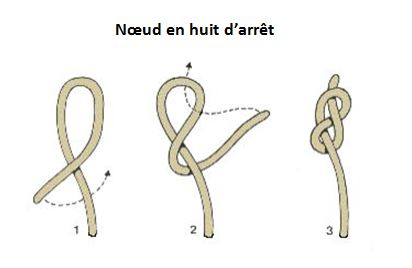
The figure-eight stopper knot (or Savoie knot) is a Locking Stopper knot at the rope end. It can support heavy or variable loads (shocks).
It is highly visible (bulky) and difficult to untie.
The figure-eight stopper knot is the safest standard for activities like climbing because it is simple to tie, offers a low risk of error, and has a symmetrical shape that allows for quick verification.
Note that this knot has an equally secure variant : the Double figure-eight knot. This latter knot, being bulkier, is rarely used in climbing as a Stopper knot.
The steps are as follows (see Figure above, cf. [MIS]) :
1. Pass the Running end over the Standing strand to form a small loop.
2. Make a complete loop around the Standing strand.
3. Pass the Running end through the loop from above (not from underneath).
4. Pull on both strands to tighten and form the figure-eight shape.
D8.1.2. Overhand knot :
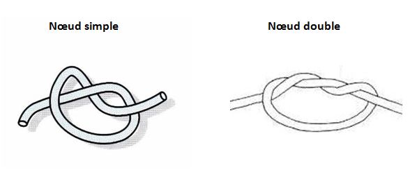
The overhand knot is a Locking Stopper knot at the rope end, under light and constant loads (without shocks).
It is discreet (not bulky), simple to tie but difficult to untie (see Figure above).
Warning : This knot is unstable if it is not tight enough.
The double overhand knot is a variant of the overhand knot by passing the Running end twice through the loop, equivalent to a double-turned Capuchin knot (see Figure above).
It is simple to tie, stronger than the simple knot and less sensitive to imperfect tightening, but more difficult to untie.
Warning : This knot is unstable if it is not tight enough.
D8.1.3. Surgeon's knot :
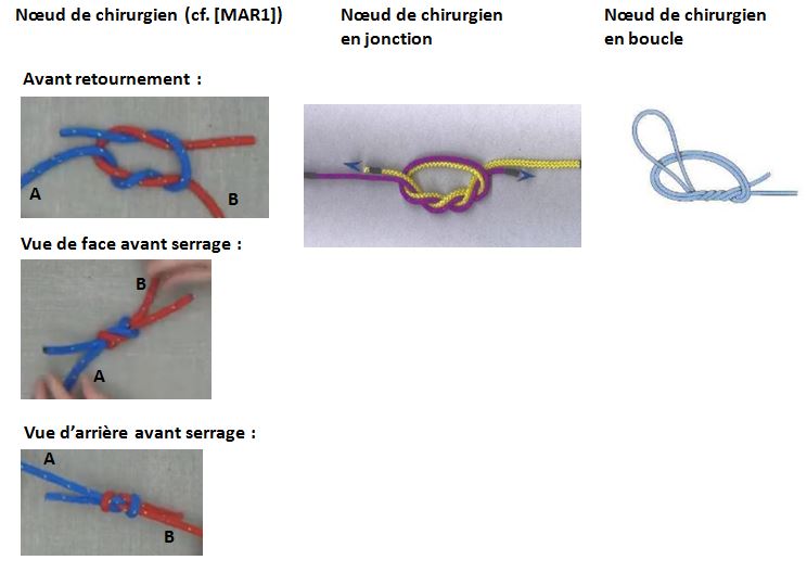
The surgeon's knot is a Locking Stopper knot used to maintain tension between two sutures. It can support heavy or variable loads (shocks).
It is complex to tie and almost impossible to untie.
This knot is a variant of the Reef knot in which the first single turn of strand A around strand B is replaced by several successive turns, similar to the Capuchin knot (see Figure above, cf. [MAR1]). This modification increases friction and strengthens the knot.
Warning : This knot is unstable if incorrectly tied in steps 3, 5 and 6.
The steps are as follows, more complex than for the Reef Knot (see Figure above, cf. [MAR1][MAR2]) :
1. Identify a reference strand (A) and pass it over the other strand (B), the two strands forming a pair of horns.
2. Make two complete loops of strand A around B and reform the pair of horns.
3. Pass strand A over strand B again and make a second complete turn around B. Warning : If the crossing is made behind strand B instead of in front, the knot will be misaligned ("granny knot") and will come undone completely when you pull on the two long strands.
4. Check that the knot has two interlocking loops, with both strands of each loop passing either under or over the strand of the opposite loop.
5. Gently pull on both standing strands to "Capsize the knot" [MAR2]. Warning : Check the correct "Capsizing" as follows : 1. Front view : two diagonal, parallel strands pass through the center of the knot, 2. Back view : two loops appear at the ends of the knot.
6. Pull firmly on both pairs of strands to tighten the knot.
D8.1.4. Prusik hitch :
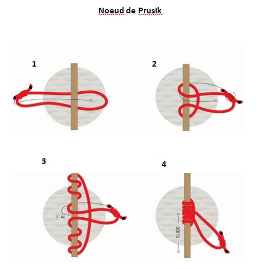
The Prusik knot is a Semi-sliding Friction knot made with a loop of cord wrapped around a main rope. It slides freely when unloaded and locks automatically under load in a symmetrical manner (in both directions of traction along the main rope), making it a simple and reliable system for climbing, rescue, or working at height.
It can support heavy or variable loads (shocks) but then becomes difficult to untie because of the tightly packed coils.
The Prusik knot is the most commonly used self-locking knot in climbing because it is simple to tie, offers a low risk of error, and has a symmetrical shape that allows for quick verification.
The steps are as follows (see Figure above, cf. [THE]) :
1. Use a cord closed into a loop (usually with a Double fisherman's knot) and position it on the main rope to form two sections : a short one and a long one.
2. Hold the short section and wrap the long section around the main rope, passing through the space between the main rope and the short section.
3. Continue wrapping, making several turns, always in the same direction and ensuring that each turn is tight around the main rope.
4. Pull gently on the long section to compress the turns against each other.
5. For added security, attach a carabiner to the long section forming the movable loop supporting the load, in order to connect it to your equipment or harness.
D8.1.5. Zeppelin bend :
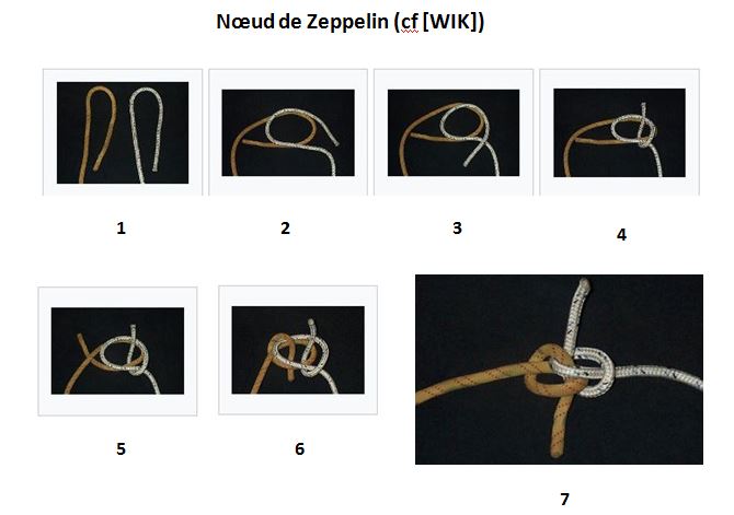
The Zeppelin bend (or Rosendahl bend) is a Locking Bend knot. It allows you to join two ropes of the same diameter under heavy or variable loads (shocks).
It is simple to tie, offers a low risk of error, and has a symmetrical shape that allows for quick verification.
It has two distinct advantages that other Bend knots do not :
- It can be loaded before being fully tightened, which allows it to be used in situations where the load changes before final tightening.
- It is very easy to untie, even after supporting significant loads.
The Zeppelin knot, like the Double fisherman's knot, is the most secure Bend knot for ropes of the same diameter (but not for ropes of different diameters).
It is often preferred to the Double fisherman's knot for the two aforementioned advantages.
There are several methods for tying this knot. The steps of the so-called "symmetric" method are as follows (see Figure above, cf. [WIK, Zeppelin Knot]) :
1. Form two identical Bights, oriented in the same direction.
2. Overlap the two Bights head-to-tail (180 ).
3. Take the Running end of the top Bight and cross it over its standing strand.
4. With this Running end, wrap it around both strands, passing underneath and emerging from the loop on the top.
5. Take the Running end of the other Bight and cross it under its standing strand.
6. With this Running end, wrap it around both strands, passing over and emerging from the loop on the bottom.
7. Tighten gradually and evenly by alternately pulling on the Running ends and then on the Standing strands.
8. Check that the knot has two parallel bars framed by two small ears, with Running ends perpendicular to Standing strands, the pattern being identical on the back side.
D8.1.6. Double overhand bend :
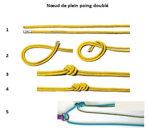
The double overhand bend is a Locking Bend knot used in climbing. It allows you to join two ropes of identical or different diameters under heavy or variable loads (shocks).
It is simple to tie and very difficult to untie.
Warning : This knot is unstable if it is not tight enough.
Thanks to its center being offset from the tension axis of the ropes, the two overhand knots compress each other at the butt without risk of twisting or slipping.
The double overhand bend is the most secure Bend knot on ropes of different diameters (and less so on ropes of the same diameter).
The steps are as follows (see Figure above, cf. [MAG1][MAG2][ARN2]) :
1. Align the two ropes parallel and in the same direction.
2. With the Running end pair, make a first Overhand knot encompassing both ropes.
3. Tighten it strand by strand by pulling successively and separately on each of the four strands. Check the symmetry of the center.
4. With the Standing end pair, make a second Overhand knot identical to the first and in the same direction. Bring this second knot against the first, then tighten it by simultaneously pulling on the two strands extending from the knot, on the side of the Standing strands.
5. Pull simultaneously and in opposite directions on the two Standing strands of each rope to compress the two knots against each other.
D8.1.7. Fisherman's knot :
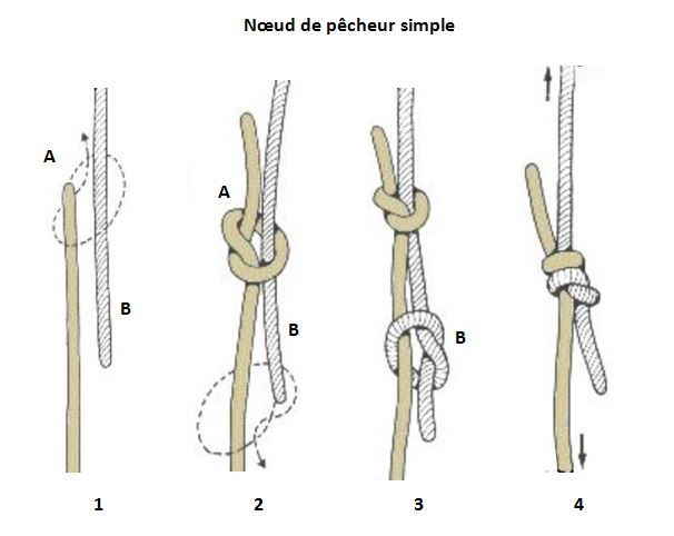
The simple fisherman's knot (or English knot) is a Locking Bend knot. It allows you to join two ropes of the same diameter under heavy or variable loads (shocks). It is particularly suitable for thin ropes.
The simple fisherman's knot is actually the assembly of two Overhand knots tightly bound together, in perfect opposition.
It is simple to tie and difficult to untie.
Warning : This knot is unstable if it is incorrectly tied at steps 3 and 4.
The steps are as follows (see Figure above, cf. [PIN][MAR3]) :
1. Place the two strands A and B head-to-tail on your work surface, with their ends overlapping.
2. With strand A, tie a Overhand knot around strand B, but not too tightly, so that the two knots can slide towards each other when tightened.
3. Rotate the assembly 180 on your work surface (this is equivalent to reversing the top and bottom) and repeat the same actions with strand B. The 180 rotation ensures proper symmetry, as the two knots will fit together and not interfere with each other at the end of the assembly.
4. Gradually pull on the two long strands to bring the two knots together, fit them into the knot, and tighten them firmly against each other.
5. Check that the knot has two parallel bars on top and two crossed X on the bottom.
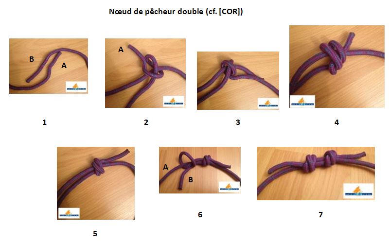
The double fisherman's knot is a variant of the simple fisherman's knot, even more secure but harder to untie.
The double fisherman's knot is actually the assembly of two Double-turn slip knots tightly bound together, in perfect opposition. Strand A wraps around strand B in the same way a Double-turn slip knot would wrap around its Standing strand.
Like the Zeppelin bend, the double fisherman's knot is the most secure Bend knot on ropes of the same diameter (but not on ropes of different diameters).
Warning :
- At the end of assembly, the two knots have the same general shape as two Double overhand knots placed side by side, but with one essential difference : End B does not pass through the loop left by A (see step 2 of the Figure "Simple fisherman's knot"), but it goes up inside the two turns (see step 4 of the Figure "Double fisherman's knot"), thus tightening the double twist more effectively.
- This knot is unstable if it is incorrectly tied at steps 6 and 7.
The steps are as follows (see Figure above, cf. [COR][MIN]) :
1. Place the two strands A and B head-to-tail on the work surface, with their ends overlapping.
2. With strand A, make a first turn around strand B, following the length of strand B towards its end and overlapping both strands.
3. Pass under B to begin the second turn, again returning towards the end of B. Both turns should be wide enough to allow a finger to pass through.
4. Complete the second turn, then pass end A through both turns.
5. Pull on the strands of the same knot, but not too tightly, so that the two knots can slide towards each other when tightened.
6. Rotate the assembly 180 on your work surface (this is equivalent to reversing the top and bottom) and repeat the same actions with strand B. The 180 rotation ensures proper symmetry, as the two knots will fit together and not interfere with each other at the end of the assembly.
7. Gradually pull on the two long strands to bring the two knots together, fit them into the knot, and tighten them firmly against each other.
8. Check that the knot has four parallel bars on top and two crossed X on the bottom.
D8.1.8. Reef knot :
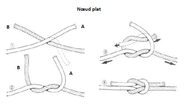
The reef knot is a Locking Bend knot. It allows you to join two ropes of the same diameter under light and constant loads (without shocks).
It is simple to tie and difficult to untie.
Warning : This knot is unstable ("granny knot") if incorrectly tied in step 3.
The steps are as follows (see Figure above, cf. [GRU]) :
1. Identify a reference strand (A) and pass it over the other strand (B), the two strands forming a pair of horns.
2. Make a complete loop of strand A around B and reform the pair of horns.
3. Pass strand A over strand B again and make a second complete turn around B. Warning : If the crossing is made behind strand B instead of in front, the knot will be misaligned ("granny knot") and will come undone completely when you pull on the two long strands.
4. Check that the knot before tightening has two interlocking loops, with both strands of each loop passing either under or over the strand of the opposite loop.
5. Pull on both pairs of strands to tighten the knot.
D8.1.9. Sheet join bend :
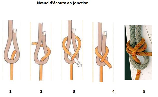
The sheet join bend (or nautical weaver's knot) is a Locking Bend knot. It allows you to join two ropes of different diameters under light and constant loads (without shocks).
It is simple to tie and difficult to untie.
Warning : This knot is unstable if incorrectly tied in steps 1 and 2.
The steps are as follows (see Figure above, cf. [SCE][DIM]) :
1. Make a wide, open loop with the thicker strand. Warning : a too small loop can cause pinching when tightening, resulting in insufficiently gradual tightening and reduced, uneven friction.
2. Pass the thinner strand under the loop and loop it completely around both thicker strands of the loop in the same direction as the initial loop formation. Warning : Reversing the direction will result in an unstable knot.
3. Unlike the Reef knot, do not pass the thinner strand back through the loop, but rather along the side between the thicker and thinner strands. Warning : check that the two short ends emerge from the same lateral side of the knot.
4. Pull on the longer strands (thick and thin) to tighten the knot.
5. Variant to secure the knot when the load is heavy (double sheet bend) : Add a second turn, passing under the thinner strand.
D8.1.10. Surgeon's join knot :

The surgeon's join knot is a Locking Bend knot used in fishing. It allows you to join two thin ropes of the same diameter, under heavy or variable loads (shocks).
It is simple to tie and difficult to untie.
This knot is a variant of the Capuchin knot, made by doubling the rope (see diagram in Surgeon's knot).
Warning : This knot is unstable if it is not tight enough.
D8.1.11. Double figure-eight knot :
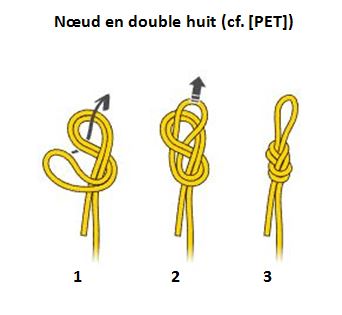
The double figure-eight knot is a Locking knot used as a Stopper knot or Hitch knot, particularly for tying up in the mountains. It can support heavy or variable loads (shocks).
It does not require an additional Stopper knot, is simple to tie and relatively error-free.
On the other hand, it is difficult to untie, especially after prolonged tension or repeated falls, which limits its use to permanent rather than temporary anchors.
This knot is a variant of the Figure-eight knot, made by doubling the rope (see Figure above, cf. [PET][ALP]).
This knot is the most secure Hitch knot on a bollard or tree type Support (but not on a ring).
In practice, however, the double figure-eight knot is not tied around a Support, as this would require pulling the entire length of rope through the loop. In fact, regardless of the Support (bolt, tree, or ring) :
A. First, form the loop at the end of the rope.
B. Make one or more Round turns around the Support with the Running end.
C. Close the knot with a connector (carabiner, quick link, etc.) linking the loop to the Standing strand, without re-tying. The anchoring is said to be "without tension" (if one or more Round turns) or "tensioned" (if only one quasi-turn of the tree).
D8.1.12. Anchor knot :

The anchor knot is a Locking Hitch knot, mainly usable on a ring or a shackle. It can support heavy or variable loads (shocks).
It is complex to tie and difficult to untie.
Its construction is similar to that of a Round turn and two half hitches, but the Half hitches are not identical : the first (a) is made on the two loops surrounding the ring, and the second (b) on the Standing strand (see Figure above, cf. [PON]).
This knot is the most secure Hitch knot on a ring (but not on a bollard or tree) because it offers optimal friction in a confined space thanks to the tight wrapping of the rope around the relatively small cross-section of the ring.
Warning : This knot is unstable if it is not tight enough.
D8.1.13. Bowline knot :
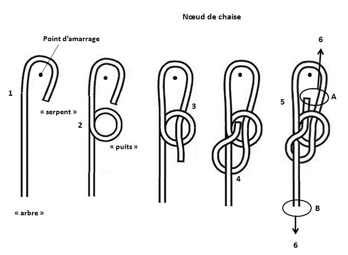
The bowline knot is a Locking Hitch knot that does not slip and can hold heavy loads under tension alone (without twisting forces, vibrations, or repeated shocks).
It is complex to tie and easy to untie, even after significant tension, making it ideal for temporary anchors.
Warning : The bowline knot can be unstable and dangerous (false bowline knot) if it is incorrectly tied in any of steps 3, 4, 5, or 6.
The steps are as follows (see Figure above, cf. [COM][ARN1]) :
Mnemonic : the snake comes out of the hole, goes around the tree, and goes back into the hole.
1. Make a large loop around the anchor point (tree, ring, etc.). The rope then has two strands :
- the Standing strand (called the "tree") which will bear the load,
- the Running end (called the "snake") which will be used to form the knot.
2. Form a loop with the tree (called the "hole") oriented towards the snake (and not towards the opposite side).
3. Place the snake at the bottom of the hole, that is, in the center of the loop and on the same side as the tree relative to the plane of the loop. Warning : If the snake is placed on the opposite side, you will get a false bowline knot.
4. The snake exits the hole and goes around the back of the tree. Warning : If the snake crosses the tree before going behind it, you will get a false bowline knot.
5. The snake enters the hole parallel to the two strands of the anchor loop, without crossing them. Warning : If the snake crosses the two strands of the loop instead of remaining parallel, you will get a false bowline knot.
6. Then tighten the knot by holding the snake and the adjacent part of the anchor loop (part A) on one side, and the tree (part B) on the other, ensuring that they are moving in opposite directions relative to the hole. Warning : Otherwise, the hole can capsize like a sock and the knot will come undone completely.
7. To prevent any accidental loosening, add a Stopper knot (Figure-eight stopper knot for example) on the Running end, close to the bowline knot.
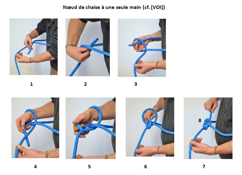
Note that this knot can be tied with one hand using a quick technique practiced in climbing.
Warning : The one-handed bowline knot can be unstable and dangerous (false bowline knot) if tied incorrectly, especially in step 6.
The steps are as follows (see Figure above, cf. [VOI][KIN][ARN1] :
1. Wrap the rope around your waist, then position the Running end over the Standing strand.
2. Rotate your wrist and make a Half hitch.
3. Turn your wrist over, palm facing up.
4. Pass the Running end under the Standing strand again, using the same hand.
5. Grasp the end and pull it over the Standing strand.
6. While holding the Standing strand with your left hand, pull the Running end of the rope through the loop where your wrist was, and reverse the knot by pulling on the Standing strand. Warning : Pull moderately, just enough to release the loop. Otherwise, the knot will be unstable or remain open.
7. Tighten the knot by pulling simultaneously on both strands (Running end and Standing strand).
8. To prevent any accidental loosening, add a Stopper knot (Figure-eight stopper knot for example) on the Running end, close to the bowline knot.
D8.1.14. Alpine Butterfly knot :
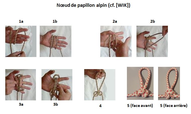
The Alpine Butterfly knot is a Locking Stopper knot, tied in the middle of the rope for intermediate anchors, tying in mid-rope, or isolating a damaged section of rope. It can support heavy or variable loads (shocks).
It is complex to tie and easy to untie, even under heavy tension.
Warning : This knot is unstable if it is incorrectly tied at any step.
There are several methods for tying this knot, including the "hand" method, which minimizes the risk of a false knot. The steps are as follows (see Figure above, cf. [WIK, Noeud de papillon alpin][SAU][NOD]) :
1. Place the rope vertically on the open palm of your hand and make three parallel turns, without overlapping the strands, working your way towards your fingers.
2. With your other hand, grasp the middle strand from underneath and pull it towards your fingers, forming a Bight.
3. Bring the Bight over the two remaining strands in your hand, wrap it around them, and bring it out again towards your fingers.
4. Remove your hand from the turns and tighten the knot firmly by pulling symmetrically on the Bight and the two strands extending from the rope.
5. Before loading, check that the knot has two small tabs on the front face and a well-formed X on the back face, which after loading transform into a flattened X on the front face and two parallel bars on the back face.
A variant of this knot exists (cf. [AND]), where the rope is placed behind the open palm of the hand (and not in front). The resulting knot is identical but with the left/right strands reversed.
D8.1.15. Clove hitch :
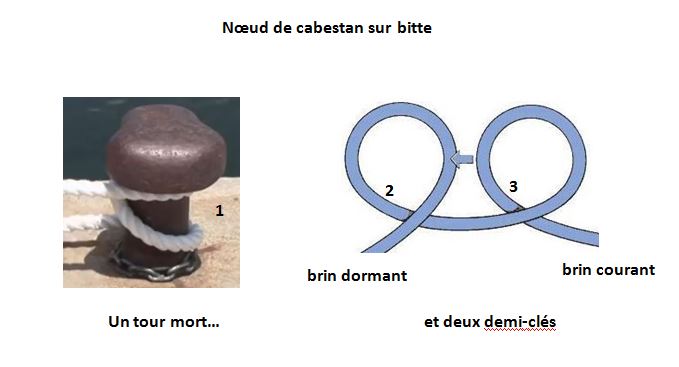
The clove hitch is a Semi-sliding Hitch knot on a bollard and a Locking Hitch knot on a tree or a ring. It allows you to secure a rope under tension to a fixed point, such as a hitch bollard.
It can support heavy constant loads (without shocks) on a bollard and variable (shocks) on a tree or a ring.
It is simple to tie and easy to untie.
Warning : This knot is unstable if incorrectly tied in steps 2 and 3.
On a bollard, the steps are as follows (see Figure above, cf. [ENA][ANI][NAU]) :
1. Make a Round turn around the bollard to absorb the rope tension and stabilize it [ENA]. This step is strongly recommended before tying the clove hitch itself (subsequent steps).
2. Form a first horizontal loop (Half hitch), passing the Running end under the Standing strand (ANI][NAU) and stacking it on the bollard.
3. Form a second horizontal loop in the same way as the first [ANI][NAU] and stack it on the bollard, creating the characteristic crossed shape of the clove hitch. Note that this second loop then appears reversed compared to the first. This is because the formation method (Running end under Standing strand), repeated twice, visually reverses the direction of the two loops.
4. Form a third loop and stack it on the bollard to secure the assembly in case the Standing strand becomes slack.

Note that this knot can be tied around a fixed point with no free end, such as a tree or a ring.
Warning : This knot is unstable if incorrectly tied in steps 2 and 3.
The steps are then as follows (see Figure above, cf. [LYO][QUE, timecode 18:30]) :
1. The Round turn around the tree is unnecessary in this situation because the first tight turn in the next step (step 1) is sufficient to absorb the rope tension and stabilize it.
2. Make a first complete loop around the tree (Half hitch), passing the Running end under the Standing strand. Tip : To keep this loop tight while making the second loop, it's best to temporarily wedge the Running end between the tree and the Standing strand, rather than simply placing it geometrically "under" the Standing strand [QUE, timecode 18:30].
3. Cross the Running end over the Standing strand and then make a second loop identical to the first.
4. Pull on the Running end to tighten the knot.
D8.1.16. Round turn and two half hitches :
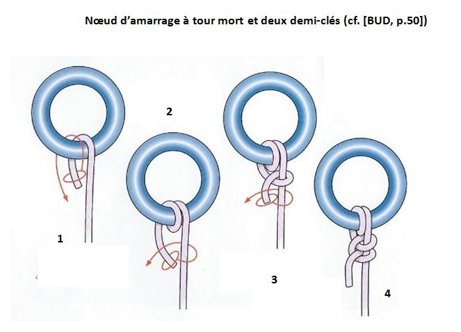
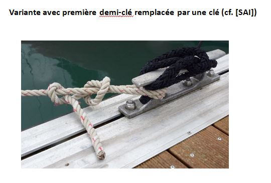
The round turn and two half hitches is a Locking Hitch knot, usable on any external Support (bollard, tree, ring, etc.). It can support heavy or variable loads (shocks).
This knot is simple to tie, relatively error-free and difficult to untie.
Its tying is similar to that of a Clove hitch, with a preliminary Round turn, but the two Half hitches are made on the Standing strand and not on the bollard (see Figure on the left above, cf. [BUD, p.50]).
This difference means that the Half hitches work by wrapping and tightening on the Standing strand, and not by constricting around the bollard, which provides a better locking under load and also greater aptitude for variable loads (shocks).
For hitching on a bollard, the round turn and two half hitches is more secure than the Clove hitch because it is fully Locking and not Semi-sliding.
This knot has several variants, including :
- Variant with only one Half hitch ("Half hitch after a round turn").
- Variant with first Half hitch replaced by a Complete hitch (see Figure on the right above, cf. [SAI]).
D8.1.17. Constrictor knot :
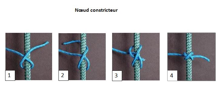
The constrictor knot is a Locking Hitch knot. It can support heavy or variable loads (shocks).
It is a variant of the Clove hitch around a tree, much tighter.
It is simple to tie and almost impossible to untie.
Warning : This knot is unstable if incorrectly tied in steps 1 and 2.
The steps are as follows (see Figure above, cf. [WIK, Noeud constricteur]) :
1. Make a complete turn around the tree, passing the Running end under the Standing strand.
2. Make a second turn, passing the Running end over the Standing strand and then under the first turn.
3. Pull on the Running end to tighten.
D8.1.18. Surgeon's loop knot :

The Surgeon's loop knot is a Locking Hitch knot used to pull a load. It can support heavy or variable loads (shocks).
This knot is a variant of the Capuchin knot, made by doubling the rope (see diagram in Surgeon's knot).
Warning : This knot is unstable if it is not tight enough.
D8.1.19. Paddle hook knot :
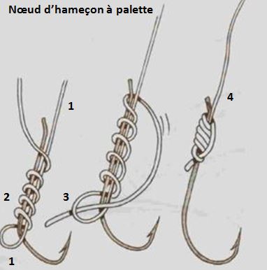
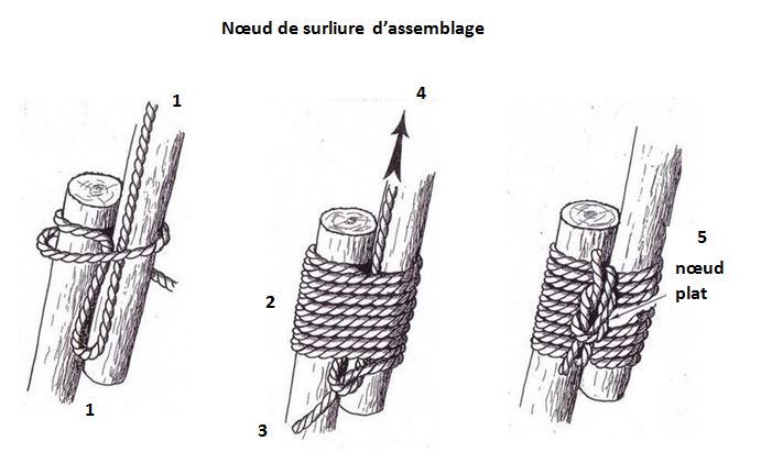
The paddle hook knot is a Locking Hitch knot, used in light fishing, which allows a fishing line to be attached along a paddle hook (without an eye), ensuring good alignment of the line with the paddle.
It is simple to tie, relatively error-free and difficult to untie.
It supports light and constant loads (without shocks).
Its construction is identical to that of the Whipping assembly knot on two parallel logs acting as a hook shank.
The steps are as follows (see Figures above, cf. [PEC]) :
1. Lay the line (or the rope) along the hook shank, making a loop on the side opposite the paddle, with a sufficiently long tail at the end.
2. Hold the loop firmly between your thumb and forefinger, then wrap the tail around the hook shank, from the loop towards the paddle, making about ten tight, close turns. In the case of a whipping assembly knot, traditional ropework often involves a reverse wrap (working towards the loop), which is still acceptable but offers less tensile strength [SCO].
3. Hold the last turn between your thumb and forefinger, then pass the free strand through the loop.
4. Pull simultaneously and fermly on both strands to tighten the knot.
5. In the case of a whipping assembly knot, for added strength, tie the two strands together with a Reef knot [SCO].
D8.1.20. Multi-turn slip knot :
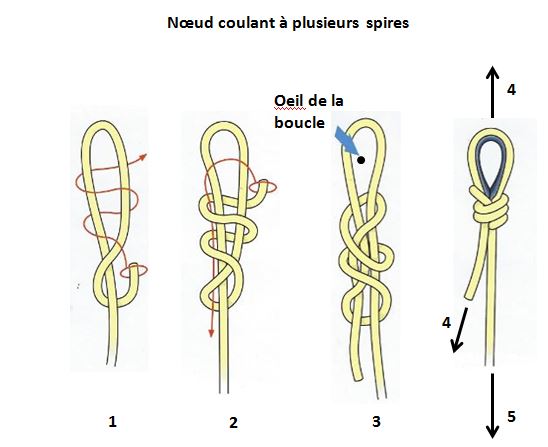
A multi-turn slip knot is a Sliding Hitch knot that automatically tightens around an object when pulled. It can support heavy or variable loads (shocks).
It is simple to tie, relatively error-free and difficult to untie.
The steps are as follows (see Figure above, cf. [BUD, p. 62][KIM]) :
1. Make a loop with the Running end and then bring it back to the base of the loop by wrapping it around the Standing strand.
2. With the Running end, wrap the two strands of the base of the loop with several tight turns, working upwards towards the eye of the loop. The turns should be wide enough to allow a finger to pass through.
3. From the eye, pass the Running end under all the turns so that it comes out on the side of the Standing strand.
4. Pull on the loop and the Running end to tighten and compact the turns, keeping them tightly closed.
5. Pull on the Standing strand or apply a load, in order to tighten the loop around the object.
D8.1.21. Lasso knot :
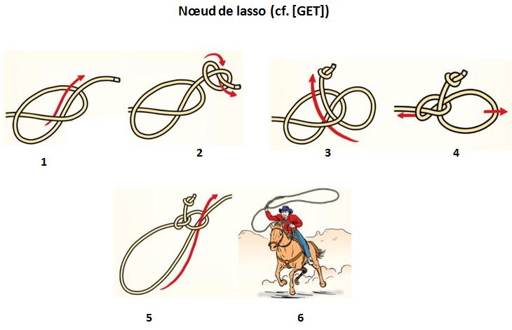
A lasso knot (or Honda knot) is a Sliding Hitch knot that automatically tightens around an object when pulled. It can support heavy or variable loads (shocks).
It is complex to tie and difficult to untie.
Warning : This knot is unstable if it is not tight enough.
The steps are as follows (see Figure above, cf. [GET][WHY]) :
1. 60 cm from the end of the rope, tie a loose Overhand knot, leaving the loop loose.
2. At the end of the rope, tie a tight Overhand knot, which will serve as the Stopper knot.
3. Pass this Stopper knot through the loose loop by inserting it through the small oval opening located between the outgoing and incoming ends of the loop, then bring it out the other side. This automatically creates a small outer loop that will be the lasso's sliding loop.
4. Tighten firmly the loose loop against the Stopper knot to lock the assembly.
5. Pass the main rope through the small loop, leaving a large outer loop that will be the lasso loop.
6. Hold the lasso loop in your dominant hand, swing it above your head with a smooth, steady motion, aim at the target, and then throw the loop so that it wraps around the target. Then pull on the main rope to tighten the loop and lock the target.
D8.1.22. Barrel sling knot :

The barrel sling knot is a Sliding Hitch knot used to safely lift a cylindrical load in a vertical position (such as a barrel). It can support heavy or constant loads (without shocks).
It is complex to tie, relatively error-free and difficult to untie.
The steps are as follows (see Figure above, cf. [KNO]) :
1. Lay a large loop on the ground, forming a Figure-eight stopper knot.
2. Place the barrel on the main strand, in the center of the loop.
3. Raise the two Running ends vertically on either side of the barrel.
4. Tie the Running ends together with a secure Bend knot (usually a Double fisherman's knot) on the side of the barrel to prevent it from being crushed by the suspended load.
5. Test the tension before fully lifting.
D8.1.23. Whipping assembly knot :
The Whipping assembly knot is a Locking Lashing knot which allows to join two parallel poles together or to consolidate a fracture on a tool handle.
It supports light and constant loads (without shocks).
It is complex to tie and difficult to untie.
Warning : This knot is unstable if it is not tight enough.
Its construction is identical to that of the Paddle hook knot (see steps and associated Figure).
D8.1.24. Diagonal lashing :
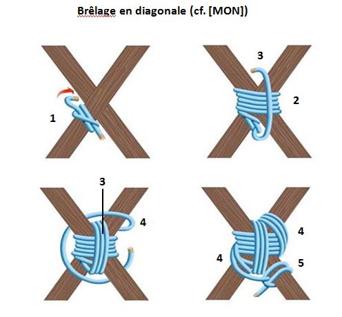
Diagonal lashing is a Locking Lashing technique used to join two parallel logs that intersect at any angle (acute, right, or obtuse). It can support heavy constant tensions (without shocks).
It is complex to tie and difficult to untie.
Warning : This knot is unstable if the turns overlap or it is not tight enough.
The steps are as follows (see Figure above, cf. [MON][REG][QUE]) :
0. Create a flat surface on the logs at the joint to prevent them from rolling.
1. Tie a Clove hitch on one of the logs (starting point).
2. Wrap the two logs diagonally with three tight turns of rope, ensuring that the strands are parallel and do not overlap.
3. Repeat this process on the other diagonal. These two sets of turns form the characteristic cross of the diagonal lashing.
4. Wrap the contact area of the two logs with three turns of rope perpendicular to the diagonal turns.
5. Finish with a Clove hitch on one of the two logs to secure the lashing.
6. Add a Stopper knot (often a Figure-eight stopper knot) to the free strand of the final clove hitch to prevent accidental loosening.
D8.1.25. Windsor necktie knot :
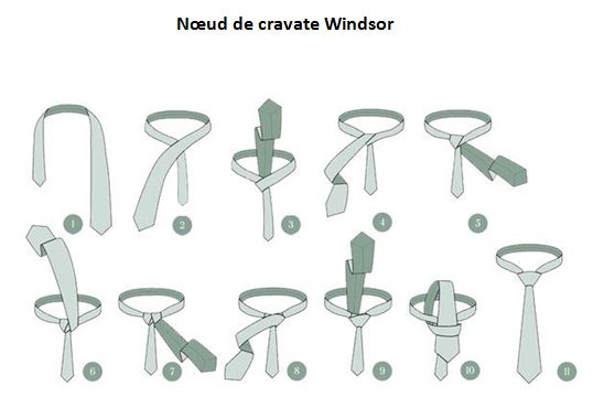
The Windsor necktie knot is a Locking Decorative knot. It is an elegant and voluminous knot, shaped like a solid, symmetrical triangle without any frills. This knot requires a long tie made of thin fabric.
It is complex to tie, relatively error-free and easy to untie.
The steps are as follows (see Figure above, cf. [CRA]) :
Mnemonic : One turn around each loop and one turn around both loops.
1. Place the tie around your collar, with the wide strand to your left and the narrow strand slightly above your navel.
2. Cross the wide strand over the narrow strand.
3. Bring the wide strand up and pass it through the loop around your neck.
4. Bring the wide strand down to your right (first turn around your neck).
5. Bring the wide strand behind the knot, to your left.
6. Bring the wide strand up again and pass it through the loop around your neck.
7. Bring the wide strand down to your left (second turn around your neck).
8. Bring the wide strand forward over the knot, to your right (turn around the two previous turns).
9. Bring the wide strand up for the third time and pass it through the loop along your neck.
10. Insert the wide strand into the front loop formed at the front of the knot.
11. Tighten the knot by gently pulling on the wide strand, then adjust it to give it a symmetrical, triangular shape.
D8.1.26. Chinese square knot :
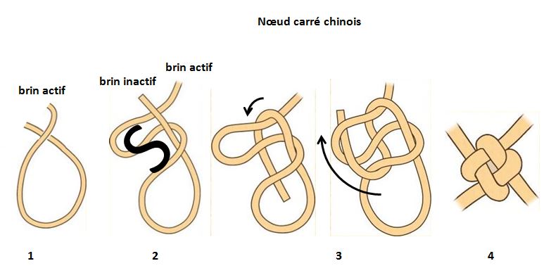
The Chinese square knot is a Locking Decorative knot that can be attractively tied on a scarf.
It is complex to tie, relatively error-free and difficult to untie.
The steps are as follows (see Figure above, cf. [SCC][CRE][DAR]) :
1. Cross one of the two strands of the scarf (called "active strand") over the other strand (called "inactive strand").
2. With the active strand, form an S with two inverted loops and three parallel segments, the bottom segment passing over the inactive strand and the other two under.
3. Pass the inactive strand under the three segments of the S, then over the S, and insert it into the top loop of the S.
4. Adjust the knot by pulling successively on the four ends of the strands.
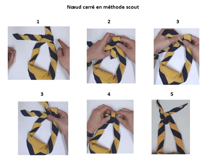
Note that this knot can be tied on oneself using another technique practiced in scouting.
The steps are as follows (see Figure above, cf. [DAR]) :
1. Cross one of the two strands of the scarf (called the "active" strand) over the other strand (called the "inactive" strand) at a 90 angle, and wrap it around.
2. Place your finger under the knot behind the inactive strand and wrap it back, forming a loop around your finger.
3. Continue wrapping the inactive strand around and bring it to the front.
4. Pass the active strand through the loop in place of your finger.
5. Adjust the knot by gently pulling on the four ends of the strands.
D8.1.27. French whipping :
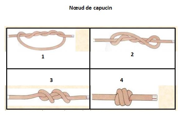
The French whipping is a Semi-sliding Decorative knot, also used as a handle or as a weight on a rope. It can support heavy or variable loads (shocks).
It is simple to tie and difficult to untie.
Warning : This knot is unstable if it is incorrectly "Capsized" or insufficiently tightened.
The steps are as follows (see Figure above, cf. [SCA]) :
1. Make an Overhand knot, passing the Running end through the loop several times.
2. Pull on both opposite ends to "Capsize the knot.
3. Continue pulling until the knot is completely tight.
4. Check that the knot appears as a cylinder of tightly packed turns.
Note that a double-turned capuchin knot is equivalent to the Double simple knot.
D8.2. How to coil a rope :
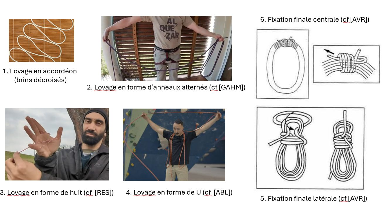
A rope is well coiled not when it is stored, but when it deploys without resistance.
Six technical choices determine how to coil a rope [PER][CHA] :
1. Coiling location :
- On the ground : To be avoided. The rope can develop kinks.
- Suspended (shoulders or hand) : Recommended. The rope stays free-flowing due to its own weight.
2. Preparation before coiling :
Before coiling, let the rope run free by hanging it loosely, so it returns to its natural state, without twist or tangle. Otherwise, all defects will be locked into the coil.
3. How to grasp the rope :
This choice determines the speed of coiling and the regularity of the winding.
- Grasping both ends together : Allows fast and regular coiling. Ensure beforehand that the rope is not twisted.
- Grasping one end only : Necessary when one end is engaged or tied.
4. The rope's natural lay ("twist") :
A laid rope has a natural lay. The coiling gesture must respect the rope's lay, i.e. never oppose the natural helical twist of the rope. In general, each loop must be formed by simple bending of the rope, without parasitic twist, with one controlled exception: the alternating wrist twist in the alternating rings coiling method described below.
5. Winding shape :
This choice determines the ease of uncoiling without twists. To achieve this characteristic, coil the rope either in accordion style (left/right alternation of curvature, see Figure 1 above), or in smart circles (alternating wrist twists), and avoid plain circles (all in the same direction) that accumulate twist.
5.1. Smart circles coiling (alternating rings, see Figure 2above) : Uncoiling is immediate and twist-free, provided the rope is thrown allowing loops to run free. Technique : Hold one rope end in one hand. With the other hand, form a loop over the previous one, stacking rings. For each new loop, give the wrist a half-turn in the opposite direction from the previous. Thus warning, one loop receives a twist, the next the inverse twist. The introduced torsion couples cancel pairwise during uncoiling.
5.2. Figure-eight coiling (accordion composed of figure-eight loops, see Figure 3 above) : The alternation is purely geometric, without wrist movement. Uncoiling is immediate and twist-free. Different techniques are possible :
A. Technique between two fingers for fine ropes (cf. [RES, 9:00]) : Trap the rope between index and middle finger of the same hand. Pass the rope alternately around the thumb and pinky to alternate figure-eight loops. The central crossing is always on the same side.
B. Thumb-to-arm technique for short ropes (cf. [JAS]) : Same technique as (A), but between the thumb and the upper arm near the elbow, initially holding one end of the rope in the hand.
C. Neck-to-wrist technique for long ropes (cf. [OUT]) : Same technique as (A), but between the neck and the wrist, initially holding one end of the rope in the hand.
5.3. U-shape coiling (accordion composed of equal-length back-and-forth loops, shoulders as gauge, see Figure 4 above) : Uncoiling is immediate and twist-free.
Pendulum technique (cf [ABL]) : The rope is laid loosely on the ground to one side, with one end held in the right hand. Grasp the hanging rope on the right with the left hand between thumb and index finger, then spread the arms apart while letting the rope slip through the left hand. Pass the loop behind the neck and release the rope from the right side. Then grasp the hanging rope on the left with the right hand between thumb and index finger, spread the arms apart while letting the rope slip through the right hand. Pass the loop behind the neck and release the rope from the left side. Repeat the process, alternating left and right.
5.4. Note : For figure-eight and U coiling methods, it is the left/right alternation of the curvature imposed on the rope at each pivot that cancels twist during uncoiling. The crossing of the strands between the pivots is an unavoidable consequence of this : clearly visible in the figure-eight coiling (between the two pivots), and more discreet in the U-shaped coiling (behind the neck between the two hands).
6. Final coiling fixation :
This choice determines deployment speed and subsequent transport.
- Lateral fixation (encircling the coil, see Figure 5 above) : Quick to undo, suited for immediate use. Technique (cf [ABL]) : With the free end, make several tight turns around the coil's body, at mid-height of the coil stack, ensuring turns are adjacent without overlap. Then, with the free end, form a bight pulled to the other side of the coil, under the turn belt just formed. Pass the free end through the bight and tighten.
- Central fixation (at coil midpoint, see Figure 6 above) : Longer to undo, but allows shoulder-carrying without coil sagging. Technique (cf [ABL]) : Central fixation follows the same principle as lateral: a turn belt around the coil locked by a bight. It differs only in position (bight at coil midpoint rather than perimeter) and execution order (bight captured in belt during formation rather than locking a pre-formed belt).
|
Summary : The most error-tolerant coiling method - both for human mistakes and rope defects - is the pendulum U-shape coiling, which is the only coiling method that self-corrects during execution. In this method : - The loops hang freely on both sides of the neck, - Their weight naturally puts the rope under vertical tension, - This tension continuously helps eliminate residual micro-twists. The other methods mentioned above are more technical : - The smart circles coiling requires constant wrist discipline. - Figure-eight coiling requires a very precise gesture : each loop must be formed correctly to avoid the progressive accumulation of residual twist. |
D8.3. Glossary :
Bight = Loop of a rope in the shape of an elongated U, without crossing the strands.
Capsizing of a knot = Step that occurs after several turns of one strand around another, as in the case of the French whipping and the Surgeon's knot. By simultaneously pulling on the Standing strands, the turns reorganize around the central part of the knot, which compacts the whole, changes the geometry of the knot, and increases its internal friction.
Complete hitch (rare term with no universal definition) = Overhand knot whose loop completely encircles the Support, which may be external or internal.
Half hitch = Nautical knot consisting, after making a turn around any object, of passing the end of the Running end under the standing part. The object may be an external Support (bollard, tree, ring) or internal (outgoing Standing strand).
Half hitch after a round turn = Hitch knot with a Round turn and a single Half hitch.
Main use =
- Stopper knots = Used to block the end of a rope and prevent fraying or slipping.
- Friction knots (or self-locking knots) = Used to allow a rope to slide freely without a load, while ensuring automatic locking under load.
- Bend knots = Used to join two ropes together.
- Hitch knots = Used to attach a rope to a fixed point (bollard, tree, ring, etc.).
- Lashing knots (or rigid joining knots) = Used to tie two rigid objects together (poles, logs, etc.) using a rope.
- Decorative knots = Used to create aesthetic patterns.
Munter (or Italian) hitch = Friction knot on a carabiner.
Round turn = Complete turn of a rope around a Support before the Running end crosses the starting point (Standing strand), which, in practice, often makes one and a half turns around the circumference of the Support (see Clove hitch).
Running end = Free end of the rope that is manipulated to form the knot.
Standing strand = Fixed part of the rope that remains still during the knot-tying process and bears the load.
Support = External anchor point (bollard, tree, ring, etc.) or internal such as a part of rope (outgoing Standing strand), serving as a fixed base for winding the Running end during a Half hitch or a Complete hitch.
Tying = The ease of tying a knot is defined as its ability to be made quickly and correctly in a situation, because it relies on an elementary spatial choreography of gestures and strands.
Tightening =
- Locking knot : Locks onto the Standing strand with or without load, and slides back after being unloaded only with manual intervention (example : Figure-eight stopper knot).
- Sliding knot : Slides along the Standing strand without load, locks under load, and slides back after being unloaded only with manual intervention (example : Multi-turn slip knot).
- Semi-sliding knot : Slides along the Standing strand without load, locks under load, and slides back spontaneously (without manual intervention) after being unloaded (example : Prusik hitch).
Unstable knot = Poorly executed knot, therefore unreliable and able to untie itself spontaneously under load (without manual intervention).
Untying = The ease of untying a knot is defined as its ability to be undone after supporting a heavy load.
D8.4. Sources relating to knots :
[ABL] A BLOC, Lover une Corde : Mes 3 Techniques Préférées ! (Youtube, 05:00).
[ALP] AlpineSavvy, Using a rope to make a tensionless tree anchor.
[AND] andreba, Noeud papillon alpin (Youtube, 01:45).
[ANI] Animated knots, Clove Hitch - Loops.
[ARN1] ArnO'Voyages, [Tuto'Escalade] Le noeud d'encordement en CHAISE - Comment faire - Quelle utilisation ? (Youtube, 04:08).
[ARN2] ArnO'Voyages, [Tuto'Escalade] Le noeud de jonction - Noeud simple - descente en rappel - Comment faire ? (Youtube 02:52).
[AVR] Club d'Escalade de l'Avranchin, Lovage des cordes.
[BUD] Budworth Geoffrey, Guide des noeuds, Parragon Books Ltd, 2006.
[CHA] ChatGPT, le moteur d'Intelligence Artificielle développé par OpenAI.
[COM] comment_economiser.fr, Le Noeud de Chaise est le Noeud le Plus Utile : Solide, Facile à Faire et à Défaire..
[COR] Cordévasion, Comment faire un noeud de pêcheur double en escalade.
[CRA] E.L. Cravatte, Le noeud Windsor.
[CRE] Les Créatifs, Nouage : une boucle chinoise.
[DAR] Dargis Pierre, Noeud carré (Youtube, 02:05).
[DIM] Dimitri Elledge, Comment faire le noeud d'écoute (+noeud d'écoute double) - Noeud de jonction! (Youtube, 04:45).
[ENA] Enautic, Le Noeud : 1 tour mort et 2 demi clés (Youtube, 00:54).
[FRA] La fraternité du scoutisme, Assemblage du bois.
[GAHM] Groupe Alpin de Haute Montagne, Lover une corde, un anneau de cordelette, une sangle (Youtube, 06:55).
[GET] gettin, A Cool Guide demonstrating how to Tie a Lasso.
[GRU] Grupo Scout Barrio La Victoria, Nudo rizo.
[JAS] Jason's Knot Channel, A Simple Trick Everyone Who Uses Rope Should Know! | How to Coil Rope & Paracord (Youtube, 05:57).
[KIM] kimoc13, Faire le noeud coulant facilement. (Youtube, 04:30).
[KIN] KINRED, Faire le noeud de chaise avec une main les yeux fermés ! (Youtube, 00:23).
[KNO] knots.neocities.org, Figure 8 Barrel sling.
[LYO] http://lyon.noeuds.free.fr, Les noeuds - Le noeud de cabestan.
[MAG1] Montagnes Magazine, Bien choisir son noeud pour rabouter 2 cordes.
[MAG2] Montagnes Magazine, Comment faire un noeud de jonction de corde ?.
[MAR1] Marsala, Noeud de chirurgien (Youtube, 01:39).
[MAR2] Marsala, Matelotage : Noeud de chirurgien (Youtube, 01:18).
[MAR3] Marsala, Noeud de pecheur simple.MOV (Youtube, 02:08).
[MIN] Minute Forme, Réaliser un noeud double pêcheur (Youtube, 01:57).
[MIS] La Misaine, Noeuds marins.
[MON] Orientacion en el campo y tecnicas de Montanismo - Nudos, amarres y estructuras.
[NAU] Nautisme-pratique.com, le noeud cabestan.
[NOD] Nodo Farfalla (Alpine Butterfly Knot): Tutorial(Youtube, 00:33).
[OUT] outdoorinstruction, Fast Coiling a Long Rope (Youtube, 05:06).
[PEC] Pêche pro, Les noeuds.
[PER] Perplexity, le moteur d'Intelligence Artificielle développé par Perplexity AI.
[PET] Petzl, Noeuds.
[PIN] Pinterest, Noeud marin.
[PON] Pontonniers de Genève, Cordages.
[QUE] Le Quercus, Les Noeuds de brêlages (Youtube, 25:08).
[REG] Regroupement scout francophone 64e Clarence-Rockland, Brêlage en croix.
[RES] Comment lover toutes les cordes! #bushcraft #survie (Youtube, 12:54).
[SAI] True Sailor, Noeud tour-mort deux demi-clés.
[SAU] Sauvetage Rivière Boréal, 8 noeuds utiles pour le sauvetage en eau vive et en eaux vives.
[SCA] Science Maison, Noeud de capucin.
[SCC] Science Maison, Noeud carré décoratif.
[SCE] Science Maison, Noeud d'écoute (oeud de tisserand).
[SCO] ScoutWiki, Surliure.
[THE] The Knots Manual, How to Tie a Prusik Knot.
[VOI] Voile & Moteur, Matelotage : Variations sur noeud de chaise.
[WHY] WhyKnot, Apprenez à nouer un lasso de cow-boy (Youtube, 01:49).
[WIK] Wikipedia, Noeud constricteur.
[WIK] Wikipedia, Noeud de papillon alpin.
[WIK] Wikipedia, Noeud de Zeppelin.
 Last page update : June 12, 2026.